Standardizing Ubiquitination Quantification: From Foundational Principles to Cross-Tissue Applications in Research and Drug Development
This article provides a comprehensive roadmap for researchers, scientists, and drug development professionals aiming to standardize the quantification of ubiquitination across diverse tissue types.
Standardizing Ubiquitination Quantification: From Foundational Principles to Cross-Tissue Applications in Research and Drug Development
Abstract
This article provides a comprehensive roadmap for researchers, scientists, and drug development professionals aiming to standardize the quantification of ubiquitination across diverse tissue types. We explore the foundational role of ubiquitination in cellular processes and disease, with examples from cervical and ovarian cancer. The piece critically evaluates current high-throughput methodologies—including TUBE-based assays, APEX2 proximity labeling, DIA mass spectrometry, and HiBiT/NanoBRET systems—highlighting their application in proteomics, drug discovery for PROTACs, and immune microenvironment analysis. A dedicated troubleshooting section addresses tissue-specific challenges and optimization strategies for detection sensitivity and specificity. Finally, we outline robust validation frameworks involving independent prognostic analysis, cross-platform verification, and single-cell RNA sequencing to ensure data reliability and translational potential for biomarker discovery and therapeutic development.
Ubiquitination Fundamentals: Decoding a Key Regulatory Mechanism in Health and Disease
Core Mechanism of the Ubiquitin-Proteasome System
What is the ubiquitin-proteasome system (UPS) and its primary function?
The Ubiquitin-Proteasome System (UPS) is the primary pathway for selective protein degradation in eukaryotic cells, responsible for maintaining cellular protein homeostasis (proteostasis) [1] [2]. This highly conserved system eliminates short-lived, misfolded, damaged, and regulatory proteins, thereby controlling vital cellular processes including immune response, apoptosis, cell cycle, differentiation, and signaling [3] [4]. The UPS functions as a hierarchical process where proteins are first tagged with ubiquitin chains and then degraded by the proteasome [3].
What are the key steps in the E1-E2-E3 enzyme cascade?
The process of ubiquitination involves a three-step, ATP-dependent enzymatic cascade [5] [6]:
- Step 1: Ubiquitin Activation (E1)
- Step 2: Ubiquitin Conjugation (E2)
- Step 3: Ubiquitin Ligation (E3)
After initial ubiquitination, additional ubiquitin molecules are attached to internal lysines on the previously attached ubiquitin, forming polyubiquitin chains that mark the protein for degradation by the 26S proteasome [5].
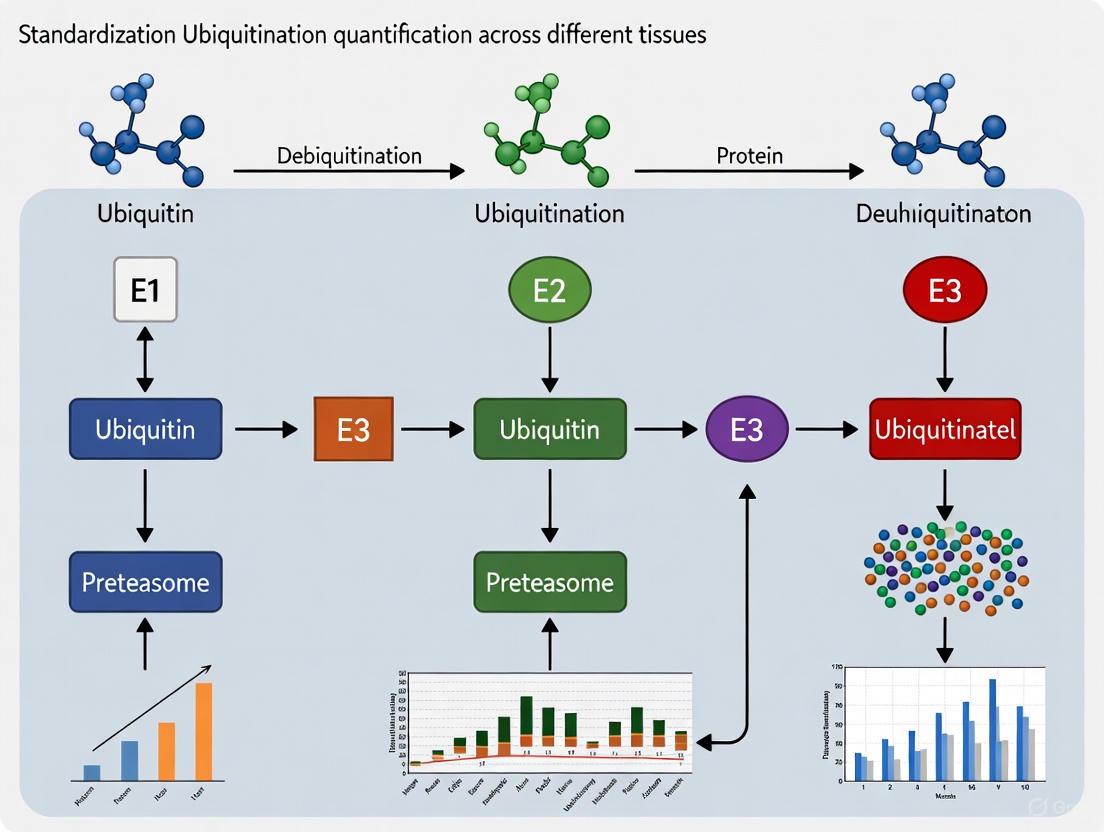
Diagram 1: The E1-E2-E3 enzyme cascade in the Ubiquitin-Proteasome System. Ubiquitin is sequentially activated by E1, conjugated to E2, and finally ligated to the target protein by E3, forming a polyubiquitin chain that targets the protein for proteasomal degradation.
Frequently Asked Questions (FAQs)
What different types of ubiquitin chains exist and what are their functions?
Ubiquitin contains seven internal lysine residues (K6, K11, K27, K29, K33, K48, K63) and an N-terminal methionine (M1) that can form polyubiquitin chains with distinct functions [3] [7] [4]. The specific linkage type determines the functional consequence for the modified protein, creating a complex "ubiquitin code" [4].
Table 1: Major Ubiquitin Linkage Types and Their Primary Functions
| Linkage Type | Primary Function | Cellular Process |
|---|---|---|
| K48-linked | Proteasomal degradation [3] [7] | Protein turnover, homeostasis [3] |
| K11-linked | Proteasomal degradation, ERAD [3] | Cell cycle regulation, protein quality control [3] |
| K63-linked | Signal transduction, protein trafficking, DNA repair [7] | NF-κB and MAPK signaling, inflammation [3] [7] |
| M1-linked | Inflammatory signaling [4] | NF-κB activation, immune regulation [4] |
| K27/K29-linked | Proteasomal and lysosomal degradation [3] | Protein quality control, autophagy [3] |
How does UPS dysfunction contribute to human diseases?
Dysregulation of UPS components is implicated in numerous human diseases [3] [4]:
- Cancer: Stabilization of oncogenes or degradation of tumor suppressors due to altered E3 ligase or deubiquitinase (DUB) activity [3] [4].
- Neurodegenerative Diseases: Impaired clearance of toxic protein aggregates (e.g., α-synuclein in Parkinson's, Huntingtin in Huntington's, amyloid-β in Alzheimer's) [1] [4].
- Immune Disorders: Aberrant inflammatory signaling due to disrupted ubiquitination of immune regulators like RIPK2, NEMO, and inflammasome components [3] [7].
- Developmental Disorders: Mutations in DUBs and E3 ligases causing congenital developmental defects [4].
- Diabetes: UPS involvement in insulin signaling, β-cell function, and pyroptosis regulation [8].
What are the therapeutic applications of targeting the UPS?
Several therapeutic strategies exploit the UPS:
- PROTACs (Proteolysis Targeting Chimeras): Heterobifunctional molecules that recruit E3 ligases to target specific disease-causing proteins for degradation [3] [6] [7]. This approach can target previously "undruggable" proteins [7].
- Molecular Glues: Small molecules that enhance the interaction between E3 ligases and target proteins [3].
- Proteasome Inhibitors: Drugs like bortezomib that globally inhibit proteasome activity, used in multiple myeloma treatment [3].
- DUB Inhibitors: Compounds targeting deubiquitinating enzymes to modulate ubiquitin-dependent signaling [7].
Troubleshooting Common Experimental Issues
How can I detect and quantify protein ubiquitination?
Detecting protein ubiquitination presents challenges due to the dynamic nature of this modification and the potential for rapid deubiquitination. The following protocol and troubleshooting guide addresses common issues.
Table 2: Troubleshooting Guide for Ubiquitination Detection
| Problem | Possible Cause | Solution |
|---|---|---|
| Weak or no ubiquitin signal | Rapid deubiquitination by DUBs during lysis | Use DUB inhibitors (e.g., N-ethylmaleimide) in lysis buffer [7] |
| Low abundance of ubiquitinated species | Treat cells with proteasome inhibitor (MG132) to accumulate ubiquitinated proteins [5] | |
| Inefficient immunoprecipitation | Use TUBEs (Tandem Ubiquitin Binding Entities) for higher affinity capture [7] | |
| Non-specific bands | Antibody cross-reactivity | Validate antibodies with ubiquitin knockout cells; use linkage-specific TUBEs [7] |
| Incomplete blocking | Optimize blocking conditions; use different blocking buffers (BSA vs. milk) [9] | |
| Cannot distinguish specific ubiquitination | Global ubiquitination changes mask target | Use chain-specific TUBEs (K48 vs. K63) to detect linkage-specific ubiquitination [7] |
| High background | Antibody concentration too high | Titrate primary and secondary antibodies; increase wash stringency [9] |
Protocol: Linkage-Specific Ubiquitination Detection Using TUBEs
Purpose: To specifically capture and detect endogenous K48- or K63-linked ubiquitination on target proteins.
Reagents Needed:
- Chain-specific TUBEs (K48-TUBE, K63-TUBE, Pan-TUBE)
- Proteasome inhibitor (MG132, 10-20µM)
- Appropriate cell lysis buffer with DUB inhibitors
- Antibodies for target protein and ubiquitin
- Magnetic beads for pull-down
Procedure:
- Cell Treatment & Lysis:
- Treat cells with experimental conditions (e.g., L18-MDP for K63 ubiquitination or PROTAC for K48 ubiquitination) [7].
- Pre-treat with proteasome inhibitor for 4-6 hours before harvesting to accumulate ubiquitinated proteins [5].
- Lyse cells in optimized buffer (e.g., 50mM Tris-HCl pH7.5, 150mM NaCl, 1% NP-40, 1mM EDTA) containing fresh DUB inhibitors (1mM N-ethylmaleimide) and protease inhibitors [7].
Ubiquitin Capture:
- Incubate 200-500µg of cell lysate with chain-specific TUBE-conjugated magnetic beads (1-2µg TUBE/100µg lysate) for 2-4 hours at 4°C with rotation [7].
- Include controls with Pan-TUBE and opposite chain-specific TUBE.
Washing and Elution:
- Wash beads 3-4 times with lysis buffer containing 300-500mM NaCl to reduce non-specific binding.
- Elute bound proteins with 2X SDS sample buffer at 95°C for 10 minutes.
Detection:
- Analyze by Western blotting with target protein-specific antibody.
- Confirm ubiquitination with anti-ubiquitin antibody.
Diagram 2: Experimental workflow for linkage-specific ubiquitination detection using TUBEs. Cell lysates are prepared with DUB inhibitors and incubated with different chain-specific TUBEs in parallel to capture distinct ubiquitin linkage types.
How do I troubleshoot poor Western blot results for UPS components?
Common Western blot issues and solutions for UPS proteins:
- Smeared Bands: Run gel at lower voltage (10-15V/cm); check for overloading; ensure proper sample preparation [10].
- High Background: Decrease antibody concentration; optimize blocking buffer; increase wash stringency; use Tween-20 in buffers [9].
- Weak Signal: Confirm efficient transfer using reversible protein stain; increase protein loading; use higher sensitivity substrate [9].
- Multiple Non-specific Bands: Validate antibody specificity; check for protein degradation (use fresh protease inhibitors) [9].
The Scientist's Toolkit: Key Research Reagents
Table 3: Essential Research Reagents for UPS Studies
| Reagent Type | Specific Examples | Function/Application |
|---|---|---|
| Proteasome Inhibitors | MG132, Bortezomib, Carfilzomib | Accumulate ubiquitinated proteins by blocking proteasomal degradation [5] |
| DUB Inhibitors | N-ethylmaleimide, PR-619 | Prevent deubiquitination during sample processing [7] |
| Chain-Specific TUBEs | K48-TUBE, K63-TUBE, M1-TUBE | High-affinity capture of linkage-specific polyubiquitin chains [7] |
| Ubiquitin Activation Inhibitors | PYR-41, TAK-243 | Inhibit E1 enzyme to block global ubiquitination [6] |
| E1/E2/E3 Enzymes | Recombinant UBE1, UBE2D2, E3 ligases | In vitro ubiquitination assays; enzyme activity studies [6] |
| Linkage-Specific Antibodies | Anti-K48-ubiquitin, Anti-K63-ubiquitin | Detect specific ubiquitin chain types by Western blot [7] |
| PROTAC Molecules | RIPK2 PROTAC, ARV-110, ARV-471 | Induce targeted protein degradation for functional studies [3] [7] |
| Activity Assays | LanthaScreen Conjugation Assay | High-throughput screening of ubiquitin conjugation [5] |
The ubiquitin code represents a sophisticated post-translational modification system that regulates nearly all cellular processes through diverse chain topologies. Ubiquitin is a small, highly conserved protein of 76 amino acids that can be covalently attached to substrate proteins via a sequential enzymatic cascade involving E1 activating, E2 conjugating, and E3 ligase enzymes [11]. This modification can take various forms, including monoubiquitination or polyubiquitination, where additional ubiquitin molecules are attached to one of the eight possible lysine residues (K6, K11, K27, K29, K33, K48, K63) or the N-terminal methionine (M1) of the previously conjugated ubiquitin molecule [12] [13]. The specific linkage type determines the downstream fate and function of the modified protein, creating a complex "ubiquitin code" that cells utilize to regulate signaling pathways, protein degradation, and immune responses [11].
The functional specialization of different ubiquitin linkages represents a crucial mechanism for cellular regulation. Among the homotypic ubiquitin chains, K48-linked polymers are predominantly associated with targeting proteins for proteasomal degradation, thereby regulating signal transduction, cell division, stress response, and development [13]. In contrast, K63-linked chains are primarily involved in non-proteolytic functions including inflammatory signaling, lymphocyte activation, and DNA repair processes [7] [11]. The remaining homotypic polyubiquitin chains are collectively classified as atypical and continue to be intensively studied for their specialized cellular roles [13]. Furthermore, recent research has revealed the existence and functional significance of heterotypic branched ubiquitin chains, such as the K48-K63 branched chain that regulates NF-κB signaling by modulating reader protein recognition and deubiquitinase sensitivity [14]. This complex architecture enables highly dynamic and precise regulation of cellular processes, with disruptions in ubiquitin signaling contributing to various diseases including cancer, neurodevelopmental disorders, and inflammatory conditions [15] [16].
Functional Roles of Different Ubiquitin Linkages
Table 1: Functional diversity of ubiquitin chain linkages
| Linkage Type | Chain Length | Primary Functions | Cellular Processes |
|---|---|---|---|
| K48 | Polymeric | Targeted protein degradation [11] | Signal transduction, cell division, stress response [13] |
| K63 | Polymeric | Signal transduction, protein trafficking [7] | Immune responses, inflammation, lymphocyte activation [11] |
| K6 | Polymeric | DNA repair, antiviral responses [11] | Autophagy, mitophagy [11] |
| K11 | Polymeric | Cell cycle progression [11] | Proteasome-mediated degradation [11] |
| K27 | Polymeric | DNA replication [11] | Cell proliferation [11] |
| K29 | Polymeric | Wnt signaling downregulation [11] | Neurodegenerative disorders, autophagy [11] |
| M1 (Linear) | Polymeric | Cell death and immune signaling [11] | NF-κB activation, inflammatory responses [13] |
Specialized Functions and Signaling Roles
Beyond the classical K48 and K63 linkages, research continues to reveal specialized functions for less common ubiquitin chain types. K11-linked chains have been implicated in cell cycle progression and can also target proteins for proteasomal degradation, similar to K48 linkages [11]. K29-linked ubiquitination has been associated with neurodegenerative disorders and participates in the downregulation of Wnt signaling pathways [11]. M1-linked linear ubiquitin chains play crucial roles in regulating cell death and immune signaling, particularly in the activation of NF-κB pathways [11].
The functional diversity of ubiquitin chains is further expanded through the formation of branched ubiquitin chains with complex topologies. Recent studies have identified significant biological roles for heterotypic ubiquitin chains, such as the K48-K63 branched chain that regulates NF-κB signaling [14]. In response to interleukin-1β, the E3 ubiquitin ligase HUWE1 generates K48 branches on K63 chains formed by TRAF6. These branched linkages create a unique ubiquitin code that permits recognition by TAB2 while simultaneously protecting K63 linkages from CYLD-mediated deubiquitylation, thereby amplifying NF-κB signals [14]. This mechanism demonstrates how ubiquitin chain branching can differentially control readout of the ubiquitin code by specific reader and eraser proteins to activate specific signaling pathways.
Experimental Protocols for Ubiquitin Chain Analysis
Determining Ubiquitin Chain Linkage Using Mutant Ubiquitins
Table 2: Key reagents for ubiquitin linkage determination experiments
| Reagent | Function/Description | Working Concentration |
|---|---|---|
| E1 Enzyme | Ubiquitin-activating enzyme | 100 nM [12] |
| E2 Enzyme | Ubiquitin-conjugating enzyme | 1 μM [12] |
| E3 Ligase | Ubiquitin ligase (substrate-specific) | 1 μM [12] |
| Wild-type Ubiquitin | Full-length ubiquitin with all lysines | ~100 μM [12] |
| Ubiquitin K-to-R Mutants | Single lysine to arginine mutants | ~100 μM [12] |
| Ubiquitin K-Only Mutants | Single lysine-only mutants | ~100 μM [12] |
| MgATP Solution | Energy source for enzymatic reaction | 10 mM [12] |
| 10X E3 Ligase Reaction Buffer | Reaction conditions maintenance | 1X final concentration [12] |
A critical methodology for determining ubiquitin chain linkage involves utilizing ubiquitin lysine mutants in in vitro ubiquitin conjugation reactions [12]. This protocol requires performing two sets of nine parallel reactions each. The first set utilizes seven ubiquitin Lysine-to-Arginine (K-to-R) mutants, where each mutant lacks a specific lysine residue. The conjugation reaction containing the ubiquitin K-to-R mutant missing the lysine required for chain linkage will be unable to form chains, resulting in only mono-ubiquitination observable by Western blot [12]. For example, if ubiquitin chains are linked via K63, all reactions except the one containing the ubiquitin K63R mutant will yield ubiquitin chains.
The second verification set utilizes seven ubiquitin K-Only mutants, where each ubiquitin mutant contains only one lysine with the remaining six mutated to arginine. In this system, ubiquitin chains formed with a specific ubiquitin K-Only mutant must utilize the single available lysine for linkage [12]. Following the K63 linkage example, only reactions containing wild-type ubiquitin and the ubiquitin K63 Only mutant will yield ubiquitin chains. This systematic approach enables robust identification of the specific lysine residues involved in ubiquitin chain formation.
Diagram 1: Experimental workflow for determining ubiquitin chain linkage using ubiquitin mutants. This two-step approach utilizes both K-to-R and K-Only mutants for robust linkage identification.
Mass Spectrometry-Based Ubiquitin Chain Analysis
Mass spectrometry-based approaches provide powerful alternatives for ubiquitin chain analysis. The Ub-AQUA/PRM (ubiquitin-absolute quantification/parallel reaction monitoring) method enables direct and highly sensitive measurement of the stoichiometry of all eight ubiquitin-ubiquitin linkage types simultaneously [17]. This targeted proteomics approach takes advantage of the characteristic di-glycine (-GG) modification left after tryptic digestion of ubiquitin incorporated in a chain [18]. By quantifying these topology-characteristic peptides, researchers can determine the relative abundance of each ubiquitin chain topology within a proteome.
The Ub-AQUA/PRM protocol involves several critical steps: stabilization of ubiquitin chains during cell lysis through the use of proteasome inhibitors (e.g., MG-132) and deubiquitinase inhibitors; preparation of heavy isotope-labeled peptide standards corresponding to each ubiquitin linkage type; tryptic digestion of protein samples; and parallel reaction monitoring mass spectrometry analysis [18]. This method allows for global assessment of ubiquitin topology landscape changes in response to cellular stimuli or perturbations, providing a comprehensive view of ubiquitin chain dynamics in biological contexts.
Technical Support Center: Troubleshooting Guides and FAQs
Frequently Asked Questions
Q: Why does my ubiquitin Western blot show a smeared appearance instead of discrete bands?
A: The smeared appearance is actually expected and indicates successful capture of ubiquitinated proteins. Since the Ubiquitin-Trap binds monomeric ubiquitin, ubiquitin polymers, and ubiquitinylated proteins, the bound fraction contains proteins of varying molecular weights, resulting in a continuous smear on the gel [11]. Discrete bands would suggest a very specific, homogeneous ubiquitination event, which is uncommon.
Q: Can ubiquitin traps differentiate between different ubiquitin linkages?
A: Standard ubiquitin traps like the ChromoTek Ubiquitin-Trap are not linkage-specific and will bind multiple different chain types [11]. Differentiation between bound linkages requires subsequent analysis using linkage-specific antibodies during Western blotting or utilizing chain-specific TUBEs (Tandem Ubiquitin Binding Entities) that are designed with nanomolar affinities for specific polyubiquitin chains [7].
Q: How can I increase or protect protein ubiquitination signals in my samples?
A: Ubiquitination signals can be preserved and enhanced by treating cells with proteasome inhibitors such as MG-132 prior to harvesting [11]. A recommended starting point is incubation with 5-25 μM MG-132 for 1-2 hours, though conditions should be optimized for specific cell types. Note that overexposure to MG-132 can lead to cytotoxic effects, so time course and dose-response experiments are advised.
Q: What are the limitations of using mutant ubiquitins for linkage determination?
A: While powerful, the mutant ubiquitin approach may not accurately represent all modifications involving wild-type ubiquitin, particularly for complex branched chains [7]. Additionally, this method typically requires in vitro reconstitution of the ubiquitination cascade, which may not fully recapitulate cellular conditions. Complementary approaches like mass spectrometry or TUBE-based methods may be necessary for comprehensive analysis.
Troubleshooting Common Experimental Issues
Problem: Low ubiquitination signal in cellular assays.
Solutions:
- Pre-treat cells with proteasome inhibitors (e.g., 10-100 μM MG-132 for 4 hours) to stabilize ubiquitinated proteins [18].
- Include deubiquitinase inhibitors (e.g., N-ethylmaleimide) in lysis buffers to prevent deubiquitination during sample preparation [18].
- Optimize lysis conditions using buffers specifically designed to preserve polyubiquitination [7].
- Confirm efficient immunoprecipitation using positive control ubiquitin chains (commercially available K48, K63, and M1-linked chains) [18].
Problem: Inconclusive results from ubiquitin mutant linkage experiments.
Solutions:
- Include both K-to-R and K-Only mutant sets for complementary verification [12].
- Ensure proper negative controls by replacing MgATP with dH₂O to confirm ATP-dependence of reactions [12].
- Verify enzyme concentrations and activity, particularly E3 ligase functionality.
- Consider the possibility of mixed or branched linkages if all single K-to-R mutants still produce chains [12].
Problem: High background in ubiquitin pulldown experiments.
Solutions:
- Increase stringency of wash conditions (higher salt concentrations, detergents).
- Use loBind tubes to prevent non-specific protein adsorption [18].
- Include control beads without ubiquitin-binding entities.
- Optimize binding conditions and input protein amounts to avoid overloading.
Advanced Methodologies: TUBEs and Branched Chain Analysis
The development of Tandem Ubiquitin Binding Entities (TUBEs) has revolutionized the study of linkage-specific ubiquitination in cellular contexts. TUBEs are specialized affinity matrices with nanomolar affinities for polyubiquitin chains that facilitate precise capture of chain-specific polyubiquitination events on endogenous proteins [7]. These reagents can be employed in high-throughput screening assays to investigate ubiquitination dynamics in response to various stimuli.
Recent applications demonstrate how chain-specific TUBEs can differentiate context-dependent ubiquitination. In studies of RIPK2, a key regulator of inflammatory signaling, K63-TUBEs specifically captured L18-MDP-induced K63 ubiquitination, while K48-TUBEs captured RIPK2 PROTAC-induced K48 ubiquitination [7]. This specificity enables researchers to dissect complex ubiquitination events occurring on the same protein in different signaling contexts.
For analyzing complex ubiquitin architectures like branched chains, the Ub-AQUA/PRM method has been adapted to quantify K48/K63 branched ubiquitin chains specifically [17]. Additionally, the Ub-ProT (ubiquitin chain protection from trypsinization) method enables measurement of ubiquitin chain length on specific substrates through combination of a chain protector and limited trypsin digestion [17]. These advanced methodologies provide researchers with powerful tools to decipher the complexity of ubiquitin networks in cellular regulation.
Diagram 2: K48-K63 branched ubiquitin chain signaling pathway in NF-κB activation. This branched topology creates a unique code that enhances signal transduction.
Research Reagent Solutions
Table 3: Essential research reagents for ubiquitination studies
| Reagent Category | Specific Examples | Applications | Providers/Sources |
|---|---|---|---|
| Ubiquitin Mutants | K-to-R mutants, K-Only mutants | Linkage determination, chain formation analysis [12] | Boston Biochem, R&D Systems [12] |
| Chain-Specific TUBEs | K48-TUBEs, K63-TUBEs, Pan-TUBEs | Linkage-specific enrichment, endogenous protein analysis [7] | LifeSensors [7] |
| Ubiquitin Traps | Ubiquitin-Trap Agarose, Ubiquitin-Trap Magnetic Agarose | General ubiquitin pulldowns, protein isolation [11] | ChromoTek [11] |
| Positive Control Chains | K48-linked chains, K63-linked chains, M1-linear chains | Method validation, standard curves [18] | Boston Biochem [18] |
| Mass Spec Standards | Heavy labeled -GG peptides | Ub-AQUA/PRM quantification [18] | JPT Peptide Technologies [18] |
| Inhibitors | MG-132 (proteasome), NEM (DUB) | Signal stabilization, pathway inhibition [18] | Multiple commercial sources |
This comprehensive toolkit enables researchers to address diverse questions in ubiquitin biology, from basic linkage determination to complex cellular signaling studies. The selection of appropriate reagents depends on the specific research goals, whether studying global ubiquitin chain topology changes, investigating ubiquitination of specific proteins, or dissecting the functional consequences of specific ubiquitin linkages in signaling pathways.
Core Biomarker Findings in Ovarian and Cervical Cancer
This section summarizes key quantitative findings from recent studies on ubiquitination-related biomarkers in ovarian and cervical cancer.
Table 1: Prognostic Ubiquitination-Related Gene Signature in Ovarian Cancer
| Aspect | Description | Performance/Findings |
|---|---|---|
| Gene Signature | 17-gene ubiquitination-related prognostic model [19] [20] | - |
| Predictive Performance | Area Under Curve (AUC) for survival prediction [19] [20] | 1-year AUC: 0.7033-year AUC: 0.7045-year AUC: 0.705 |
| Clinical Outcome | Overall Survival (OS) between risk groups [19] [20] | High-risk group: Significantly lower OS (P<0.05) |
| Immune Microenvironment | Immune cell infiltration in low-risk group [19] [20] | Higher levels of CD8+ T cells (P<0.05), M1 macrophages (P<0.01), and follicular helper cells (P<0.05) |
| Key Ubiquitin Ligase | FBXO45 (E3 ligase) functional role [19] [20] | Promotes cancer cell growth, spread, and migration via Wnt/β-catenin pathway |
Table 2: Key Ubiquitination-Related Targets in Cervical Cancer
| Component | Role/Function | Experimental Findings |
|---|---|---|
| ECT2 | Guanine nucleotide exchange factor, oncogene [21] | Upregulated in CESC tissues/cells; knockdown inhibits proliferation, migration, invasion, and glycolysis |
| USP13 | Deubiquitinating enzyme (DUB) [21] | Stabilizes ECT2 by removing ubiquitin chains; high expression in cervical cancer |
| USP13-ECT2 Axis | Functional interaction [21] | USP13 inhibition suppresses cervical cancer tumor growth in vivo by promoting ECT2 degradation |
Diagram 1: USP13-ECT2 axis in cervical cancer. USP13 removes ubiquitin from ECT2, preventing its degradation and promoting oncogenic processes.
Detailed Experimental Protocols
Protocol: Constructing a Ubiquitination-Related Gene Prognostic Model
This protocol is adapted from the methodology used to develop a 17-gene prognostic signature for ovarian cancer [19] [20].
1. Data Collection and Processing:
- Obtain transcriptomic data (RNA-Seq) and corresponding clinical data (e.g., survival time, status) for ovarian cancer patients from public databases like The Cancer Genome Atlas (TCGA-OV).
- Acquire data from normal ovarian tissue samples from sources like the Genotype-Tissue Expression (GTEx) project via the UCSC Xena browser.
- Use the R package
edgeRto identify Differentially Expressed Genes (DEGs) between tumor and normal tissues. Apply a threshold of |logFC| ≥ 1 and an adjusted p-value < 0.01.
2. Candidate Gene Screening:
- Obtain a comprehensive list of ubiquitination-related genes (UBQ genes). This list can be sourced from databases such as the UUCD (Ubiquitin and Ubiquitin-like Conjugation Database).
- Intersect the UBQ gene list with the identified DEGs to find co-expressed ubiquitination-related genes.
- Perform univariate Cox proportional hazards regression analysis on the co-expressed genes to identify those significantly associated (P < 0.05) with overall survival.
3. Predictive Model Construction:
- Apply LASSO (Least Absolute Shrinkage and Selection Operator) regression analysis to the candidate genes from the Cox analysis to penalize and select the most robust predictors, reducing overfitting.
- Calculate a risk score for each patient using the formula:
Risk score = Σ(Coef_i × Expr_i), whereCoef_iis the regression coefficient from the LASSO model for each gene, andExpr_iis the gene's expression level. - Split patients into high-risk and low-risk groups based on the median risk score.
4. Model Validation:
- Assess the model's performance using Kaplan-Meier survival analysis to visualize the survival difference between the two risk groups (log-rank test p-value < 0.05 indicates significance).
- Evaluate the model's predictive accuracy using time-dependent Receiver Operating Characteristic (ROC) curve analysis, calculating the Area Under the Curve (AUC) for 1, 3, and 5-year survival.
- Validate the model's stability using an external validation cohort (e.g., from the GEO database, such as GSE165808 or GSE26712).
Protocol: Detecting Protein Ubiquitination using ThUBD-Coated Plates
This protocol describes a high-throughput method for capturing ubiquitinated proteins, offering significant sensitivity improvements over previous technologies [22].
1. Plate Coating:
- Use Corning 3603-type 96-well plates.
- Coat each well with 1.03 μg ± 0.002 of Tandem Hybrid Ubiquitin Binding Domain (ThUBD) fusion protein. This protein exhibits unbiased, high-affinity binding to all types of ubiquitin chains.
- Incubate overnight at 4°C to allow for stable adsorption of ThUBD to the plate surface.
2. Sample Preparation and Incubation:
- Lyse cells or tissues in a lysis buffer that preserves ubiquitination, typically containing protease inhibitors and deubiquitinase (DUB) inhibitors (e.g., N-Ethylmaleimide) to prevent the loss of ubiquitin signals.
- Clarify the lysate by centrifugation. Determine the protein concentration.
- Add a standardized amount of protein lysate (e.g., 5-20 μg) to each ThUBD-coated well. For target-specific ubiquitination, include a primary antibody against the protein of interest.
- Incubate the plate for 2-3 hours at room temperature with gentle shaking to allow ubiquitinated proteins to bind to the immobilized ThUBD.
3. Washing and Detection:
- Wash the wells thoroughly with a optimized washing buffer (e.g., PBS with 0.05% Tween-20) to remove non-specifically bound proteins.
- For global ubiquitination assessment: Add ThUBD-HRP (Horseradish Peroxidase) conjugate and detect the chemiluminescent signal, which is proportional to the total amount of captured ubiquitinated protein.
- For target-specific ubiquitination: After washing, add an HRP-conjugated secondary antibody specific to the primary antibody and detect via chemiluminescence.
- Quantify the signal, which is proportional to the amount of ubiquitinated protein captured. The ThUBD platform shows a 16-fold wider linear range and superior sensitivity compared to TUBE-based assays [22].
Diagram 2: ThUBD-based ubiquitination detection workflow. This high-throughput method captures ubiquitinated proteins with high affinity and specificity.
Protocol: Investigating Linkage-Specific Ubiquitination using TUBEs
This protocol is useful for differentiating between K48-linked (degradation) and K63-linked (signaling) polyubiquitin chains on a target protein like RIPK2 [7].
1. Cell Stimulation and Lysis:
- Culture relevant cells (e.g., THP-1 monocytic cells for studying RIPK2 in inflammation).
- Treat cells with a stimulus:
- To induce K63-linked ubiquitination: Treat with L18-MDP (200-500 ng/ml for 30-60 min).
- To induce K48-linked ubiquitination: Treat with a specific PROTAC (e.g., RIPK2 degrader-2).
- Lyse cells in a buffer optimized for preserving polyubiquitin chains, including DUB inhibitors.
2. Enrichment with Chain-Specific TUBEs:
- Use 96-well plates or magnetic beads coated with chain-specific Tandem Ubiquitin Binding Entities (TUBEs):
- K48-TUBEs: Specifically enrich for K48-linked polyubiquitin chains.
- K63-TUBEs: Specifically enrich for K63-linked polyubiquitin chains.
- Pan-TUBEs: Enrich for all chain types.
- Incubate the cell lysate with the TUBE-coated matrix for several hours at 4°C.
3. Analysis:
- Wash the matrix thoroughly to remove non-specifically bound proteins.
- Elute the bound ubiquitinated proteins or proceed directly to immunoblotting.
- Detect the protein of interest (e.g., RIPK2) by Western blot using a specific antibody. The appearance of a higher molecular weight smear indicates successful ubiquitination.
- The specific TUBE type used (K48 vs K63) will determine which ubiquitin linkage is visualized on the blot.
Troubleshooting Guides & FAQs
FAQ 1: What are the main advantages of the ThUBD-based detection method over traditional TUBEs?
The ThUBD (Tandem Hybrid Ubiquitin Binding Domain) platform offers two critical advantages [22]:
- Unbiased Binding: ThUBD is engineered to have high affinity for all types of ubiquitin chains (K48, K63, etc.), whereas traditional TUBEs can exhibit linkage bias, potentially skewing results.
- Enhanced Sensitivity: The ThUBD-coated plate technology demonstrates a 16-fold wider linear range and significantly improved detection sensitivity, capturing ubiquitinated proteins from complex proteome samples at levels as low as 0.625 μg.
FAQ 2: How can I distinguish between different types of ubiquitin linkages (e.g., K48 vs. K63) in my cellular experiment?
You can utilize chain-specific TUBEs in a plate-based or bead-based enrichment assay [7].
- For K63-linked ubiquitination (often involved in signaling), use K63-TUBEs. For example, L18-MDP-induced RIPK2 ubiquitination is captured effectively by K63-TUBEs.
- For K48-linked ubiquitination (associated with proteasomal degradation), use K48-TUBEs. For example, PROTAC-induced target ubiquitination is primarily captured by K48-TUBEs.
- By running your sample in parallel with different chain-specific TUBEs, you can determine the predominant linkage type modified on your target protein in a given biological context.
Troubleshooting Guide: Common Issues in Ubiquitination Assays
Table 3: Troubleshooting Common Ubiquitination Experiment Issues
| Problem | Possible Cause | Solution |
|---|---|---|
| Weak or no ubiquitination signal | Rapid deubiquitination after cell lysis; low affinity capture reagent. | Add deubiquitinase (DUB) inhibitors (e.g., N-Ethylmaleimide) directly to the lysis buffer. Use high-affinity capture reagents like ThUBD [22]. |
| High background in Western blot | Non-specific antibody binding; inefficient washing. | Include appropriate controls (e.g., no primary antibody). Optimize washing stringency (e.g., increase salt concentration, add detergent). |
| Inability to distinguish ubiquitin linkage type | Using a pan-specific ubiquitin enrichment tool. | Employ chain-specific TUBEs (K48, K63) to selectively capture different ubiquitin linkages [7]. |
| Discrepancy between biochemical and cellular ubiquitination data | Compound cannot cross cell membrane in cellular assays (CETSA). | Verify cell membrane permeability of small molecules in whole-cell assays. Use cell lysate-based assays (e.g., PTSA) as an intermediate step [23]. |
FAQ 3: My compound stabilizes the target protein in a thermal shift assay (CETSA), but I don't see corresponding ubiquitination. Why?
This discrepancy can arise from several factors [23]:
- Cellular Permeability: The compound may not efficiently cross the cell membrane to reach its intracellular target in sufficient concentration. Check the compound's physicochemical properties or use a lysate-based CETSA to bypass permeability issues.
- Assay Sensitivity: The ubiquitination assay may not be sensitive enough to detect the change. Consider switching to a more sensitive method like the ThUBD-platform [22].
- Non-Degradative Mechanism: Stabilization of a protein against thermal denaturation does not automatically mean it is being ubiquitinated. The compound might be stabilizing the protein through a mechanism that does not involve the ubiquitin-proteasome system.
The Scientist's Toolkit: Key Research Reagents
Table 4: Essential Reagents for Ubiquitination Research
| Reagent / Tool | Function / Application | Example / Note |
|---|---|---|
| ThUBD (Tandem Hybrid Ubiquitin Binding Domain) | High-affinity, unbiased capture of all ubiquitin chain types for detection and quantification [22]. | Used coated on 96-well plates for high-throughput screens; 16x more sensitive than TUBEs. |
| Chain-Specific TUBEs | Selective enrichment of proteins modified with specific ubiquitin linkages (e.g., K48 for degradation, K63 for signaling) [7]. | Critical for understanding the functional consequence of ubiquitination on a target protein. |
| HiBiT Tag / NanoBRET Systems | Real-time, live-cell quantification of protein turnover and ubiquitination dynamics [24]. | HiBiT for degradation kinetics; NanoBRET for monitoring ubiquitination events and protein-protein interactions. |
| DUB Inhibitors (e.g., N-Ethylmaleimide) | Preserve ubiquitin signals in cell lysates by inhibiting deubiquitinating enzymes that would otherwise remove ubiquitin chains [7]. | Essential additive to cell lysis buffers for all ubiquitination enrichment experiments. |
| PROTACs (Proteolysis Targeting Chimeras) | Heterobifunctional molecules that recruit E3 ligases to target proteins, inducing their ubiquitination and degradation [19] [7]. | Tool molecules for studying targeted protein degradation; RIPK2 degrader is an example. |
Ubiquitination is a critical post-translational modification traditionally known for regulating protein degradation, signal transduction, and cellular homeostasis through the attachment of ubiquitin to lysine residues on target proteins [25]. However, emerging research has revealed that ubiquitination extends beyond canonical protein targets to include non-protein substrates such as saccharides and metabolites. This expansion, termed non-canonical ubiquitination, represents a frontier in understanding the diverse regulatory mechanisms controlling metabolic pathways, immune responses, and cellular signaling networks. The study of these non-canonical modifications presents unique technical challenges, from detection difficulties to experimental artifacts, requiring specialized methodologies and troubleshooting approaches. This technical support center provides a comprehensive framework for standardizing ubiquitination quantification across tissue research, offering detailed protocols, troubleshooting guides, and analytical tools to advance investigations into these novel ubiquitination phenomena.
Technical Challenges in Non-Canonical Ubiquitination Research
Investigating ubiquitination of non-protein substrates presents researchers with several distinct technical hurdles that must be addressed for reliable experimentation and data interpretation.
Detection Sensitivity Issues: The primary challenge in studying non-canonical ubiquitination stems from the inherently low abundance and transient nature of these modifications. As noted in global ubiquitylation studies, ubiquitylation site occupancy spans over four orders of magnitude, with median ubiquitylation site occupancy being three orders of magnitude lower than that of phosphorylation [26]. This low stoichiometry makes detection particularly challenging for non-protein substrates where established enrichment methods may not be optimized.
Methodological Limitations: Traditional ubiquitination research tools were developed specifically for protein substrates. When applied to saccharides and metabolites, these tools often yield suboptimal results. As one resource notes, "ubiquitination signals in a sample can be preserved by treating cells with proteasome inhibitors, such as MG-132, prior to harvesting" [27]. However, the effectiveness of such stabilization methods for non-protein substrates remains inadequately characterized, requiring careful optimization for each experimental context.
Specific Technical Hurdles:
- Antibody Specificity: Many ubiquitin antibodies are non-specific and bind large amounts of artifacts [27], complicating the detection of novel modification types.
- Dynamic Range: The percentage of ubiquitinylated proteins (and presumably other molecules) in a cell lysate is often very small, requiring highly sensitive enrichment methods [27].
- Stability: The ubiquitination process is highly dynamic, rapid, and reversible [28], making capture of transient modifications particularly challenging.
Troubleshooting Guide: Common Experimental Issues and Solutions
Table 1: Troubleshooting Common Problems in Non-Canonical Ubiquitination Studies
| Problem | Possible Causes | Recommended Solutions |
|---|---|---|
| Weak or No Signal | Low modification stoichiometry; Inefficient enrichment; Incompatible detection method | Pre-treat cells with 5-25 µM MG-132 for 1-2 hours before harvesting [27]; Use chain-specific TUBEs (Tandem Ubiquitin Binding Entities) with nanomolar affinities [7]; Validate with multiple detection platforms |
| High Background Noise | Non-specific antibody binding; Inadequate blocking; Sample degradation | Use high-affinity nanobody traps (e.g., ChromoTek Ubiquitin-Trap) for cleaner pulldowns [27]; Optimize washing stringency; Include appropriate negative controls (e.g., bacterial dapB) [29] |
| Inconsistent Results Between Replicates | Variable enrichment efficiency; Protease activity; Incomplete inhibition of deubiquitinases | Standardize lysis conditions with optimized buffer to preserve polyubiquitination [7]; Include protease and deubiquitinase inhibitors; Use internal reference standards for normalization |
| Failure to Detect Linkage-Specific Modifications | Use of pan-specific detection methods only; Linkage instability | Employ chain-selective TUBEs that differentiate context-dependent linkage specific ubiquitination [7]; Combine with linkage-specific antibodies for verification |
Frequently Asked Questions (FAQs)
Q1: Can standard ubiquitin antibodies detect non-canonical ubiquitination on metabolites? Most commercially available ubiquitin antibodies were developed for protein-based applications and may have limited utility for non-protein substrates. Due to weak immunogenicity of small ubiquitin proteins and potential artifacts [27], we recommend using high-affinity capture tools like Ubiquitin-Trap combined with mass spectrometry for verification. Always validate findings with multiple methodological approaches.
Q2: How can we differentiate between K48, K63, and other linkage types on non-protein substrates? Chain-selective TUBEs can differentiate context-dependent linkage specific ubiquitination [7]. For example, K48-linked chains are specifically associated with proteasomal degradation, while K63-linked chains are primarily involved in regulating signal transduction [7]. These specialized affinity matrices facilitate precise capture of chain-specific polyubiquitination events on native molecules.
Q3: What controls are essential for validating non-canonical ubiquitination? Essential controls include: (1) Positive control probes for housekeeping genes (e.g., PPIB, POLR2A, or UBC) [29]; (2) Negative control probes (e.g., bacterial dapB) [29]; (3) Untreated samples without enrichment; (4) Specificity controls using linkage-specific tools. Proper controls should generate a score ≥2 for PPIB and ≥3 for UBC with relatively uniform signal [29].
Q4: How can we enhance the stability of non-canonical ubiquitination during sample preparation? Ubiquitination signals can be preserved by treating cells with proteasome inhibitors (e.g., MG-132) prior to harvesting [27]. While optimal conditions vary by cell type, a standard starting point is 5-25 µM MG-132 for 1-2 hours. Note that overexposure can cause cytotoxic effects, requiring careful optimization.
Experimental Protocols for Non-Canonical Ubiquitination Analysis
Protocol 1: Enrichment of Ubiquitinated Metabolites Using Ubiquitin-Trap
Principle: This protocol uses high-affinity anti-ubiquitin nanobodies coupled to agarose or magnetic beads to immunoprecipitate monomeric ubiquitin, ubiquitin chains, and ubiquitinylated molecules from cell extracts [27].
Materials:
- Ubiquitin-Trap Agarose (uta) or Ubiquitin-Trap Magnetic Agarose (utma) [27]
- Lysis, wash, dilution, and elution buffers (provided in kit) [27]
- Proteasome inhibitor (MG-132, 5-25 µM working solution) [27]
- Cell lines or tissue samples of interest
Procedure:
- Pre-treatment: Incubate cells with 5-25 µM MG-132 for 1-2 hours before harvesting to preserve ubiquitination signals [27].
- Lysis: Harvest cells and lyse using the provided lysis buffer optimized to preserve polyubiquitination.
- Preparation: Clarify lysate by centrifugation at 10,000 × g for 10 minutes at 4°C.
- Enrichment: Incubate supernatant with Ubiquitin-Trap beads for 2 hours at 4°C with gentle rotation.
- Washing: Wash beads 3-5 times with provided wash buffer under stringent conditions to reduce background.
- Elution: Elute bound ubiquitinated molecules using provided elution buffer or direct denaturation.
- Analysis: Proceed to downstream applications including mass spectrometry or western blotting.
Troubleshooting Notes:
- For over- or under-fixed tissues, adjustment of pretreatment conditions may be necessary [29].
- The Ubiquitin-Trap is not linkage specific, so differentiation between bound linkages requires subsequent analysis with linkage-specific antibodies [27].
- The bound fraction may contain molecules of varying lengths, potentially resulting in a smeared appearance on gels [27].
Protocol 2: Linkage-Specific Analysis Using TUBE-Based Assay
Principle: This protocol leverages chain-specific Tandem Ubiquitin Binding Entities (TUBEs) with nanomolar affinities for polyubiquitin chains to investigate ubiquitination dynamics in a linkage-specific manner [7].
Materials:
- Chain-specific TUBEs (K48-TUBEs, K63-TUBEs, Pan-selective TUBEs) [7]
- 96-well plates coated with appropriate TUBEs
- Lysis buffer optimized for polyubiquitination preservation
- Target-specific detection antibodies
Procedure:
- Preparation: Coat 96-well plates with chain-specific TUBEs according to manufacturer's instructions.
- Stimulation: Treat cells with appropriate stimuli (e.g., L18-MDP for K63 ubiquitination induction) [7].
- Lysis: Lyse cells in optimized buffer and clarify by centrifugation.
- Incubation: Apply lysates to TUBE-coated plates and incubate for 2 hours at 4°C.
- Washing: Wash plates thoroughly to remove non-specifically bound material.
- Detection: Detect captured ubiquitinated molecules using target-specific antibodies.
- Quantification: Analyze using appropriate plate reader or imaging systems.
Application Example: This approach has been successfully used to demonstrate that inflammatory agent L18-MDP stimulated K63 ubiquitination can be faithfully captured using K63-TUBEs or Pan-selective TUBEs but not K48-TUBEs [7].
Research Reagent Solutions
Table 2: Essential Research Reagents for Non-Canonical Ubiquitination Studies
| Reagent Category | Specific Examples | Function and Application |
|---|---|---|
| Ubiquitin Enrichment Tools | Ubiquitin-Trap Agarose/Magnetic Beads [27]; Chain-specific TUBEs (K48, K63, Pan) [7] | Immunoprecipitation of monomeric ubiquitin, ubiquitin chains, and ubiquitinylated molecules from cell extracts; Linkage-specific capture |
| Stabilization Reagents | MG-132 (proteasome inhibitor) [27]; Protease inhibitor cocktails; Deubiquitinase inhibitors | Preserve ubiquitination signals by preventing degradation and deubiquitination during sample processing |
| Detection Reagents | Ubiquitin Recombinant Antibody [27]; Linkage-specific ubiquitin antibodies; HRP-conjugated secondary antibodies | Western blot detection of ubiquitinated species with reduced cross-reactivity and artifacts |
| Control Systems | Positive control probes (PPIB, POLR2A, UBC) [29]; Negative control probes (dapB) [29] | Quality assessment of sample RNA integrity and optimal permeabilization; Background signal determination |
Standardization and Workflow Optimization
Establishing reproducible methods for quantifying non-canonical ubiquitination across tissue types requires implementation of standardized workflows and quality control measures.
Recommended Workflow:
- Sample Qualification: Run samples alongside control slides using positive and negative control probes to assess sample quality [29].
- Pretreatment Optimization: For tissues not prepared according to recommended guidelines, optimize antigen retrieval and protease digestion conditions [29].
- Ubiquitin Enrichment: Select appropriate enrichment method based on research question (pan-specific vs. linkage-specific).
- Detection and Validation: Use multiple complementary detection methods to verify findings.
- Quantification and Scoring: Implement semi-quantitative scoring guidelines appropriate for your target abundance [29].
Quality Control Metrics:
- Successful positive control staining should generate a score ≥2 for PPIB and ≥3 for UBC with relatively uniform signal throughout the sample [29].
- Negative control samples should display a score of <1, indicating low to no background [29].
- Internal consistency between technical replicates should be maintained with <20% coefficient of variation.
Visualization of Experimental Workflows
Non-Canonical Ubiquitination Analysis Workflow
Ubiquitin Linkage Signaling Pathways
The investigation of non-canonical ubiquitination of saccharides and metabolites represents an emerging frontier in post-translational modification research with significant implications for understanding cellular regulation, metabolic pathways, and therapeutic development. The technical frameworks and troubleshooting guides presented here provide a foundation for standardizing research approaches across different tissue types and experimental systems. As the field advances, continued refinement of these methodologies, coupled with the development of increasingly specific research tools, will be essential for elucidating the full scope and biological significance of these non-canonical modifications. By implementing these standardized protocols and quality control measures, researchers can enhance the reproducibility and reliability of their findings, accelerating our understanding of the diverse functional roles played by ubiquitination beyond traditional protein targets.
Protein ubiquitination is a crucial post-translational modification that regulates diverse cellular functions, including protein degradation, cell signaling, and DNA repair [30]. This reversible modification involves a coordinated enzymatic cascade of E1 activating, E2 conjugating, and E3 ligating enzymes, with deubiquitinating enzymes (DUBs) providing the reverse reaction [31]. The complexity of ubiquitin signaling arises from its ability to form diverse chain topologies—including monoubiquitination, multiple monoubiquitination, and polyubiquitin chains with at least eight different linkage types—each encoding specific biological functions [30].
Studying ubiquitination across different tissue types presents substantial methodological challenges that undermine data comparability and reproducibility. The intrinsic low stoichiometry of ubiquitinated proteins, combined with the transient nature of modification and vast structural diversity of ubiquitin chains, creates significant technical hurdles [30] [32]. Furthermore, tissue-specific differences in enzyme expression, metabolic activity, and protein composition introduce additional variables that complicate cross-tissue comparisons. This technical brief establishes a standardized framework for ubiquitination research to overcome these challenges and enable robust, reproducible cross-tissue analyses.
Technical Challenges in Ubiquitination Research
Researchers face multiple interconnected challenges when investigating ubiquitination across diverse tissue samples:
- Low Abundance and Transient Nature: Ubiquitination is a highly dynamic process with rapid turnover, and ubiquitinated proteins typically represent a very small fraction of the total cellular proteome, necessitating efficient enrichment strategies [30] [32].
- Structural Complexity: Ubiquitin can form polymers with different linkage types (K48, K63, K11, K27, K29, K33, M1) that regulate distinct biological outcomes, requiring linkage-specific analytical approaches [30] [31].
- Sample Compatibility Issues: Tissue samples present unique challenges compared to cell lines, including higher protease activity, varied tissue homogenization efficiency, and differential accessibility to ubiquitination sites [33].
- Antibody Specificity Limitations: Many ubiquitin antibodies demonstrate cross-reactivity or poor affinity, leading to high background noise and non-specific binding that compromise data quality [32].
Impact on Data Reproducibility
These technical challenges manifest as substantial variability in experimental outcomes. Without standardized protocols, ubiquitination studies frequently yield irreproducible results, particularly when comparing different tissue types. Inconsistent sample preparation, enrichment methods, and analytical platforms create systematic biases that undermine data integration and meta-analysis across studies.
Standardized Methodological Framework
Optimized Sample Preparation Protocol
Standardized tissue processing is fundamental for reproducible ubiquitination analysis. The following protocol ensures sample integrity and maximizes ubiquitin recovery:
Tissue Preservation and Lysis
- Flash-freeze tissue samples in liquid nitrogen within 5 minutes of excision
- Use pre-cooled lysis buffer (8M urea, 50mM Tris-HCl pH 8.0, 150mM NaCl, 1mM EDTA) supplemented with fresh protease inhibitors (2μg/ml aprotinin, 10μg/ml leupeptin, 1mM PMSF) and 50μM PR-619 deubiquitinase inhibitor [33]
- Maintain samples at 4°C throughout homogenization using a pre-cooled dounce homogenizer
- Centrifuge lysates at 20,000×g for 10 minutes at 4°C and collect supernatant
Protein Digestion and Peptide Cleanup
- Determine protein concentration using BCA assay
- Reduce proteins with 5mM DTT (45 minutes, room temperature)
- Alkylate with 10mM iodoacetamide (30 minutes, room temperature in dark)
- Dilute lysate 1:4 with 50mM Tris-HCl (pH 8.0)
- Digest first with Lys-C (1:50 enzyme:substrate, 2 hours, room temperature)
- Follow with trypsin digestion (1:50 enzyme:substrate, overnight, room temperature)
- Acidify with 1% trifluoroacetic acid (TFA) to stop digestion
- Desalt peptides using C18 solid-phase extraction cartridges [33]
Ubiquitinated Peptide Enrichment Methods
Table 1: Comparison of Ubiquitinated Peptide Enrichment Strategies
| Method | Principle | Advantages | Limitations | Recommended Input |
|---|---|---|---|---|
| Antibody-based Enrichment | Anti-K-ε-GG antibodies recognize diGly remnant after trypsin digestion [34] | High specificity; compatible with various sample types | Potential antibody cross-reactivity; relatively high cost | 1-10mg peptide input [34] |
| Ubiquitin-Trap Technology | Ubiquitin-binding nanobody (VHH) coupled to agarose or magnetic beads [32] | Captures full ubiquitin modifications; not limited to tryptic peptides; works across species | Does not differentiate linkage types; may require secondary analysis | 0.5-2mg protein input [32] |
| Tagged Ubiquitin Systems | Ectopic expression of His- or Strep-tagged ubiquitin in cells [30] | High purification efficiency; good for cell culture studies | Not applicable to human tissues; may alter native ubiquitination | N/A (cell-based only) |
For cross-tissue studies, the automated UbiFast method provides exceptional reproducibility. This approach uses magnetic bead-conjugated K-ε-GG antibody (HS mag anti-K-ε-GG) with the following optimized workflow:
Enrichment
- Incubate 1mg peptides with 31.25μg anti-K-ε-GG antibody conjugated to magnetic beads
- Use automated magnetic particle processor for consistent handling
- Perform all steps in 1.5mL low-binding microcentrifuge tubes
- Binding time: 2 hours at 4°C with gentle rotation [33]
Washing and Elution
- Wash twice with ice-cold PBS
- Wash once with HPLC-grade water
- Elute with 0.15% trifluoroacetic acid
- Dry samples in vacuum concentrator [33]
Mass Spectrometry Analysis: DIA vs. DDA
Data-Independent Acquisition (DIA) mass spectrometry significantly outperforms traditional Data-Dependent Acquisition (DDA) for ubiquitinome analysis:
Table 2: Performance Comparison of MS Acquisition Methods for Ubiquitinome Analysis
| Parameter | DIA Method | Traditional DDA |
|---|---|---|
| DiGly peptides identified (single run) | 35,000±682 [34] | ~20,000 [34] |
| Quantitative precision (CV) | 45% of peptides <20% CV [34] | 15% of peptides <20% CV [34] |
| Data completeness | >77% of peptides across replicates [34] | ~50% missing values common [34] |
| Recommended settings | 46 precursor isolation windows\nMS2 resolution: 30,000 [34] | TopN method (N=20)\nDynamic exclusion: 30s [34] |
Optimized DIA Parameters for Ubiquitination Analysis:
- Precursor mass range: 400-1000 m/z
- Window placement: 46 variable windows optimized for diGly peptide distribution
- MS1 resolution: 120,000
- MS2 resolution: 30,000
- Normalized HCD collision energy: 28-32% [34]
Troubleshooting Guide: Frequently Encountered Issues
Low Ubiquitination Signal Detection
Problem: Weak or undetectable ubiquitination signals in tissue samples despite adequate protein input.
Solutions:
- Pre-treat tissues with proteasome inhibitors (5-25μM MG132 for 1-2 hours) before harvesting to stabilize ubiquitinated proteins [32] [34]
- Include deubiquitinase inhibitors (50μM PR-619) in lysis buffer to prevent ubiquitin removal during sample processing [33]
- Optimize antibody-to-peptide ratio (empirically determine for each tissue type)
- Increase peptide input amount (up to 2mg for difficult tissues) while maintaining proper antibody ratio
High Background and Non-Specific Binding
Problem: Excessive non-specific binding during enrichment, leading to high background and reduced specificity.
Solutions:
- Include stringent washing steps with PBS containing 0.1% SDS or deoxycholate [32]
- Use mild detergent conditions during binding (0.1% NP-40 alternative)
- Employ competitive washing with 25mM glycine (pH 2.5) for 2 minutes followed by neutralization
- Implement sequential enrichment with two rounds of antibody capture with intermediate cleaning
Inconsistent Results Across Tissue Types
Problem: Significant variability in ubiquitination detection when analyzing different tissue types.
Solutions:
- Normalize input material based on tissue-specific protein extractability rather than total protein
- Prepare tissue-specific spectral libraries to account for differential peptide detectability
- Include internal standardization with heavy labeled ubiquitin reference peptides
- Process all comparative samples simultaneously using automated platforms to minimize technical variation
Incomplete Digestion and Peptide Bias
Problem: Variable trypsin efficiency across tissue types leading to biased ubiquitin remnant representation.
Solutions:
- Standardize digestion efficiency using Lys-C/trypsin sequential digestion protocol [33]
- Monitor digestion completeness with quality control peptides
- Extend digestion time to 18-24 hours for fibrous tissues
- Incorporate chemical assist agents (Rapigest) for membrane-rich tissues
Essential Research Reagent Solutions
Table 3: Key Reagents for Standardized Ubiquitination Studies
| Reagent Category | Specific Products | Application Notes | Quality Control Requirements |
|---|---|---|---|
| Enrichment Antibodies | HS mag anti-K-ε-GG [33]; Ubiquitin-Trap Agarose/Magnetic Agarose [32] | Magnetic beads enable automation; Linkage-specific antibodies available for follow-up | Test lot-to-lot variability with reference sample; Verify specificity with ubiquitin knockout lysate |
| Enzyme Inhibitors | MG-132 (proteasome) [32]; PR-619 (DUB) [33]; Chloroacetamide (alkylating) [33] | Use fresh preparations; Optimize concentration for each tissue type | Confirm activity with fluorogenic substrate assays |
| Mass Spec Standards | TMTpro 18-plex [33]; Heavy labeled diGly reference peptides [34] | Enable multiplexing of up to 18 samples; Use for retention time alignment | Include in every run for quality control |
| Digestion Enzymes | Sequencing-grade trypsin; Lys-C [33] | Sequential digestion improves coverage; Quality varies by vendor | Verify activity with standard protein digest |
| Sample Preparation Kits | Ubiquitin-Trap Kit (includes lysis, wash, dilution, elution buffers) [32] | Standardized buffers improve reproducibility; Compatible with multiple species | Test buffer performance with control experiments |
Quality Control and Validation Framework
Implementation of Quality Control Metrics
Robust quality control measures are essential for cross-tissue ubiquitination studies:
- Process Controls: Include standardized reference tissue samples in each processing batch to monitor technical variability
- Enrichment Efficiency: Calculate K-ε-GG peptide enrichment factor by comparing pre- and post-enrichment samples
- Spectral Library Quality: Assess library completeness using target-decoy false discovery rate (FDR < 1% at peptide level) [34]
- Quantitative Reproducibility: Monitor coefficient of variation (CV) across technical replicates, targeting <20% for high-confidence identifications [34]
Data Normalization and Validation Strategies
- Cross-Tissue Normalization: Apply quantile normalization with tissue-specific adjustments for protein content variability
- Independent Validation: Confirm key findings using orthogonal methods such as Western blotting with linkage-specific antibodies or ubiquitin binding domain assays [30]
- Spike-in Controls: Use heavy labeled ubiquitin standards to correct for tissue-specific ion suppression effects [33]
Standardization of ubiquitination analysis across tissues requires implementation of consistent methodologies from sample collection through data analysis. The integrated framework presented here—encompassing standardized protocols, optimized instrumentation parameters, rigorous quality control measures, and comprehensive troubleshooting guidance—provides a foundation for generating comparable, reproducible ubiquitination data across diverse tissue types. Adoption of these standardized approaches will accelerate our understanding of tissue-specific ubiquitination signaling and facilitate the development of ubiquitin-targeted therapeutics.
High-Throughput Quantification Technologies: Tools for Precision Ubiquitinome Profiling
Tandem Ubiquitin Binding Entities (TUBEs) are engineered, high-affinity reagents designed to overcome the long-standing challenge of detecting and enriching polyubiquitinated proteins from complex biological samples. Ubiquitination, a crucial post-translational modification, regulates diverse cellular functions from protein degradation to signal transduction, with the functional outcome largely dictated by the type of polyubiquitin chain linkage formed on target proteins [35]. Unlike traditional methods such as immunoprecipitation with ubiquitin antibodies, TUBEs incorporate multiple ubiquitin-binding domains (UBDs) to achieve nanomolar affinity for polyubiquitin chains, significantly improving the capture efficiency and stability of ubiquitinated proteins during experimental procedures [35]. This technology has become indispensable for researchers studying targeted protein degradation, inflammatory signaling, and the ubiquitin-proteasome system.
The versatility of TUBE technology allows for both broad and specific analysis of the ubiquitome. Pan-selective TUBEs bind to all ubiquitin chain linkages, providing a comprehensive view of total protein ubiquitination [36] [35]. In contrast, chain-selective TUBEs offer precise tools for investigating the functional consequences of specific ubiquitin linkages, such as K48-linked chains that target proteins for proteasomal degradation or K63-linked chains involved in signal transduction and DNA repair [7] [35] [37]. This technical support document provides detailed troubleshooting guidance, experimental protocols, and FAQs to standardize the application of TUBE assays for endogenous protein analysis across different tissue types.
TUBE Selection Guide
Table 1: Characteristics and Applications of Different TUBE Types
| TUBE Type | Specificity | Key Applications | Affinity Characteristics |
|---|---|---|---|
| Pan-Selective TUBE1 | All ubiquitin linkages [35] | Comprehensive ubiquitome analysis; target-agnostic ubiquitination studies [35] | Preferentially binds K63- over K48-polyUb [36] |
| Pan-Selective TUBE2 | All ubiquitin linkages [35] | General ubiquitin pull-down; studies requiring equal affinity for major linkages [35] | Binds K48- and K63-polyUb with equal affinities [36] |
| K48-Selective HF TUBE | K48-linked chains [35] | Studying proteasomal degradation; validating PROTAC efficacy [7] [35] | High-fidelity (HF) version with ~20 nM Kd for tetra-ubiquitin [36] |
| K63-Selective TUBE | K63-linked chains [35] | Investigating NF-κB signaling, DNA repair, autophagy [7] [35] | 1,000 to 10,000-fold preference for K63-linked chains [35] |
| M1-Selective TUBE | M1-linked (linear) chains [36] | Research on NF-κB inflammatory signaling [37] | Comparable high affinity to K63 TUBE [36] |
Troubleshooting Common Experimental Issues
Problem: Low Signal in TUBE Assays
Potential Causes and Solutions:
- Insufficient Enrichment: Ensure you are using the recommended amount of cell extract. As a starting point, use 20 µL of agarose-TUBE beads or 100 µL magnetic-TUBE slurry per milligram of cell extract [36]. The amount may need optimization based on the abundance of your target protein.
- Protein Degradation: Perform all purification steps at 4°C and include a comprehensive cocktail of protease inhibitors during cell lysis to prevent deubiquitination and protein degradation [38].
- Low Abundance Target: For low-abundance endogenous proteins, consider scaling up the starting material. The high affinity of TUBEs makes them suitable for enriching scarce ubiquitinated species [39].
Problem: High Background or Non-Specific Binding
Potential Causes and Solutions:
- Insufficient Wash Stringency: Incorporate high-stringency washes. This can include increasing the NaCl concentration to 2M or greater, or adding mild detergents like 0.1% NP-40 or Tween-20 to wash buffers [38].
- Non-optimized Lysis Conditions: Vortexing lysates during preparation can cause protein complex dissociation. Avoid vortexing and use gentle pipetting instead. For some protein complexes, performing lysis in the absence of NP-40 may be necessary as they may be unstable in its presence [38].
Problem: Inability to Detect Linkage-Specific Ubiquitination
Potential Causes and Solutions:
- Incorrect TUBE Selection: Verify that you are using the appropriate chain-selective TUBE for your biological question. For example, PROTAC-induced degradation should be detected with K48-selective TUBEs, while inflammatory signaling typically involves K63-selective TUBEs [7].
- Suboptimal Cell Stimulation: Ensure proper activation of the pathway of interest. In the RIPK2 model, L18-MDP (200-500 ng/mL) stimulation for 30 minutes effectively induced K63 ubiquitination, while PROTAC treatment induced K48 ubiquitination [7].
Detailed Experimental Protocol: Analyzing Endogenous RIPK2 Ubiquitination
This protocol exemplifies the application of TUBE technology to study context-dependent ubiquitination of an endogenous protein, as demonstrated in recent research [7].
Step-by-Step Procedure
Step 1: Cell Culture and Treatment
- Culture THP-1 human monocytic cells in appropriate medium.
- For K63 ubiquitination: Treat cells with L18-MDP (200-500 ng/mL) for 30 minutes [7].
- For K48 ubiquitination: Treat cells with a specific RIPK2 PROTAC (e.g., RIPK2 degrader-2) [7].
- Include control treatments: pre-treat with Ponatinib (100 nM) for 30 minutes to inhibit RIPK2 kinase activity and suppress ubiquitination [7].
Step 2: Cell Lysis and Lysate Preparation
- Lyse cells in a lysis buffer optimized to preserve polyubiquitination. A recommended buffer should contain:
- 50 mM Tris-HCl (pH 7.5)
- 150 mM NaCl
- 1% NP-40 or Triton X-100
- Protease inhibitors (include DUB inhibitors for optimal ubiquitin preservation)
- 1 mM DTT (optional, check compatibility with your TUBE type)
- Perform lysis using freeze-thaw cycles to minimize protein complex dissociation. Avoid vortexing and trypsinizing cells [38].
- Clear lysates by centrifugation at 10,000 × g for 15 minutes at 4°C. For particularly viscous lysates due to DNA, shear genomic DNA by passing the lysate through an 18-gauge needle several times [38].
Step 3: TUBE-Based Affinity Enrichment
- For each enrichment, use 20 µL of agarose-TUBE beads or 100 µL magnetic-TUBE slurry per 1 mg of total protein [36].
- Incubate the clarified lysate with the appropriate TUBE (Pan-, K48-, or K63-selective) for 2-4 hours at 4°C with gentle rotation.
- After incubation, pellet beads magnetically or by gentle centrifugation.
Step 4: Washing and Elution
- Wash beads 3-4 times with ice-cold lysis buffer. For high background, include one wash with buffer containing 500 mM NaCl.
- Elute bound proteins using LifeSensors proprietary elution buffer (Cat # UM411B) or 2X SDS-PAGE loading buffer with heating at 95°C for 5-10 minutes [36].
Step 5: Detection and Analysis
- Analyze eluates by Western blotting using antibodies against your protein of interest (e.g., anti-RIPK2).
- For quantification, use TUBE-AlphaLISA, TUBE-DELFIA, or other HTS-compatible formats [35].
Table 2: Expected Results for RIPK2 Ubiquitination Pattern
| Experimental Condition | Pan-TUBE | K48-TUBE | K63-TUBE |
|---|---|---|---|
| Untreated Cells | Low/No Signal | Low/No Signal | Low/No Signal |
| L18-MDP Treatment | Strong Signal | Low/No Signal | Strong Signal |
| RIPK2 PROTAC Treatment | Strong Signal | Strong Signal | Low/No Signal |
| Ponatinib + L18-MDP | Low/No Signal | Low/No Signal | Low/No Signal |
Frequently Asked Questions (FAQs)
Q1: How do TUBEs compare to traditional ubiquitin antibodies for detection?
TUBEs offer significant advantages over traditional ubiquitin antibodies. They exhibit nanomolar binding affinities for polyubiquitin chains, far exceeding the affinity of most antibodies [35]. Additionally, TUBEs protect polyubiquitin chains from deubiquitinating enzymes (DUBs) and protasomal degradation during sample processing, preserving the native ubiquitination state in a way antibodies cannot [35].
Q2: Can TUBEs be used for high-throughput screening (HTS)?
Yes, TUBE technology is adaptable to HTS formats. LifeSensors offers specialized assays like the PA950 PROTAC Assay Plate for cell-based ELISA and the PA770 kit for in vitro ubiquitination assays [36]. These enable quantitative, high-throughput analysis of endogenous target protein ubiquitination, which is crucial for drug discovery programs focused on targeted protein degradation [36].
Q3: What is the difference between the PA950 and PA770 kits?
The PA950 kit is designed as a cell-based ELISA to measure ubiquitination in cellular contexts, while the PA770 kit is an in vitro based ELISA that uses pre-coated TUBE plates to capture polyubiquitin chains formed in a PROTAC-dependent reaction, allowing for precise control of reaction components [36].
Q4: How should TUBE reagents be stored and handled?
Recombinant proteins like TUBEs should generally be stored at -80°C [36]. Avoid multiple freeze-thaw cycles, as this can compromise activity. For specific storage conditions, always refer to the product datasheet available on the manufacturer's website [36].
Q5: My protein of interest is not RIPK2. Can this protocol be adapted?
Absolutely. The protocol using chain-selective TUBEs to differentiate context-dependent ubiquitination has broad applicability [7]. The key is to first understand the biological context of your protein's ubiquitination to select the appropriate TUBE (e.g., K48-TUBE for degradation studies, K63-TUBE for signaling studies) and then optimize stimulation or inhibition conditions specific to your pathway.
Research Reagent Solutions
Table 3: Essential Reagents for TUBE-Based Ubiquitination Studies
| Reagent / Material | Function / Application | Example / Notes |
|---|---|---|
| Pan-Selective TUBEs | Comprehensive capture of all polyubiquitinated proteins; ideal for initial discovery phase [35]. | TUBE1 (preferentially binds K63) and TUBE2 (equal K48/K63 affinity); available conjugated to various tags (FLAG, Biotin) and beads [36]. |
| Chain-Selective TUBEs | Precise isolation of proteins modified with specific ubiquitin linkages to determine functional outcome [7] [35]. | K48-TUBE HF (for degradation), K63-TUBE (for signaling), M1-TUBE (for linear ubiquitination in inflammation) [36]. |
| TUBE-Coated Assay Plates | High-throughput screening of ubiquitination in plate-based formats [36]. | PA950 (cell-based) and PA770 (in vitro) assay kits for quantitative analysis of PROTAC/molecular glue activity [36]. |
| Specialized Lysis Buffer | Maintains protein ubiquitination state during extraction by inhibiting DUBs and proteases [38] [7]. | Should contain protease inhibitors (including DUB inhibitors) and be compatible with downstream TUBE binding. |
| Decomplexing Buffer | Disrupts native protein complexes to reduce background and improve signal-to-noise ratio in assays [36]. | Urea-based buffer (available from LifeSensors) used prior to analysis with PA950 kit [36]. |
Ubiquitin Signaling Pathways in Physiological Contexts
Understanding the biological context of different ubiquitin linkages is crucial for designing appropriate experiments. The diagram below illustrates key pathways where specific ubiquitin linkages play definitive roles, highlighting how TUBE technology can be applied to dissect these processes.
Protein ubiquitination is a crucial post-translational modification regulating virtually all cellular processes, including protein degradation, signal transduction, and circadian biology [34] [40]. The versatility of ubiquitin signaling stems from its ability to form diverse conjugates, ranging from single ubiquitin monomers to complex polyubiquitin chains with different linkage types [41]. Disruption of ubiquitin homeostasis is linked to numerous pathologies, including cancer and neurodegenerative diseases [40] [42], making accurate quantification essential for both basic research and drug development.
A significant challenge in the field has been the lack of standardized methods capable of reliably quantifying ubiquitin pools and ubiquitination sites across diverse biological samples, particularly tissues [43] [44]. Traditional antibody-based methods have struggled to accurately discriminate between free and conjugated ubiquitin species [43]. However, recent advances combining diGly antibody enrichment with data-independent acquisition mass spectrometry (DIA-MS) now enable unprecedented depth and reproducibility in ubiquitinome mapping, offering a path toward standardized quantification across tissue types [34] [45].
Core Methodology: diGly Antibody Enrichment and DIA-MS Workflow
The foundational innovation enabling global ubiquitinome analysis was the development of antibodies specifically recognizing the diglycine (diGly) remnant left on trypsinized peptides from ubiquitinated proteins [34] [46]. When combined with advanced mass spectrometry techniques, this enrichment strategy allows system-wide profiling of ubiquitination events.
diGly Antibody-Based Enrichment
Following tryptic digestion of protein lysates, the K-ε-GG motif serves as an affinity handle for immuno-enrichment, dramatically reducing sample complexity and enabling detection of low-abundance ubiquitination events [44] [46]. This method captures endogenous ubiquitination without genetic manipulation, making it particularly valuable for tissue studies where tagged ubiquitin expression is infeasible [41] [44].
Data-Independent Acquisition Mass Spectrometry
Unlike traditional data-dependent acquisition, DIA-MS fragments all co-eluting peptides within predefined mass-to-charge windows simultaneously, resulting in more comprehensive and reproducible quantification [34] [45]. This technique significantly reduces missing values across sample series and improves quantitative accuracy, which is crucial for detecting subtle ubiquitination changes in complex tissue samples.
Table: Key Advantages of DIA-MS over DDA for Ubiquitinome Analysis
| Parameter | Data-Dependent Acquisition | Data-Independent Acquisition | Practical Benefit |
|---|---|---|---|
| Identification Depth | ~20,000 diGly peptides [34] | ~35,000-70,000 diGly peptides [34] [45] | Greater coverage of ubiquitination events |
| Quantitative Reproducibility | 15% of peptides with CV <20% [34] | 45% of peptides with CV <20% [34] | More reliable quantification across samples |
| Missing Values | High in large sample series [45] | Minimal run-to-run variability [45] | Better data completeness in tissue cohorts |
| Dynamic Range | Limited by stochastic sampling | Expanded through parallel fragmentation [45] | Improved detection of low-stoichiometry sites |
Integrated Workflow for Ubiquitinome Mapping
The complete workflow integrates sample preparation, diGly enrichment, and advanced mass spectrometry, with specific optimizations for different sample types.
Technical Performance and Optimization Guidelines
Method Performance Metrics
Recent implementations of DIA-based ubiquitinomics have demonstrated remarkable improvements in analytical performance. In single measurements of proteasome inhibitor-treated cells, DIA methods identify approximately 35,000 distinct diGly peptides—nearly double the number obtained with DDA methods [34]. With further optimization, this can be extended to over 70,000 ubiquitinated peptides in single MS runs [45].
Quantitative precision has shown similar improvements, with DIA methods achieving coefficients of variation below 20% for 45% of quantified diGly peptides, compared to only 15% with DDA [34]. This enhanced reproducibility is particularly valuable for tissue studies where biological variability necessitates robust measurement techniques.
Sample Preparation Optimization
Lysis Buffer Selection: Recent comparisons demonstrate that sodium deoxycholate (SDC)-based lysis with chloroacetamide alkylation outperforms traditional urea buffers, yielding 38% more diGly peptides while maintaining enrichment specificity [45]. SDC lysis also improves quantitative precision and is compatible with tissue samples.
Input Material Requirements: For tissue samples, 2 mg of protein input provides optimal balance between identification depth and practical feasibility, yielding approximately 30,000 diGly peptides [45]. Lower inputs (500 μg or less) substantially reduce coverage, dropping below 20,000 identifications [45].
Fractionation Strategies: For maximum depth, high-pH reversed-phase fractionation (96 fractions concatenated to 8) enables identification of >90,000 diGly peptides when combined with diGly enrichment [34]. Separating fractions containing abundant K48-linked ubiquitin chain-derived diGly peptides reduces competition during antibody enrichment and improves detection of co-eluting peptides [34].
Table: Optimized Sample Preparation Parameters for Tissue Ubiquitinomics
| Parameter | Recommended Condition | Effect on Results | Considerations for Tissues |
|---|---|---|---|
| Lysis Buffer | 5% SDC + 40mM chloroacetamide [45] | 38% increase in diGly identifications vs. urea [45] | Effective for heterogeneous tissue samples |
| Protein Input | 2 mg total protein [45] | ~30,000 diGly peptide identifications | Limited by tissue availability; can scale down |
| Enrichment Scale | 1mg peptide : 31.25μg antibody [34] | Optimal peptide yield and coverage | Consistent ratio maintains reproducibility |
| Fractionation | 96 → 8 concatenated fractions [34] | >90,000 diGly peptide library depth | Adds processing time but essential for depth |
| K48-Peptide Handling | Separate enrichment of abundant chains [34] | Reduces interference with rare peptides | Particularly important for diseased tissues |
Troubleshooting Guide: FAQs for Ubiquitinome Mapping Experiments
Q1: Our ubiquitinome coverage from tissue samples is substantially lower than reported values. What are the key areas to investigate?
- Lysis Efficiency: Verify complete tissue disruption using SDC-based lysis buffer with immediate boiling and chloroacetamide alkylation to preserve ubiquitination states [45].
- Antibody Capacity: Ensure proper ratio of peptide input to diGly antibody (1mg peptide:31.25μg antibody). Overloading dramatically reduces identification numbers [34].
- Sample Complexity: For heterogeneous tissues, consider pre-fractionation before diGly enrichment to reduce complexity and increase coverage of low-abundance ubiquitination events [34].
- Protease Inhibition: Include deubiquitinase inhibitors during tissue processing to prevent loss of ubiquitin chains before analysis [43].
Q2: We observe high variability in ubiquitinated peptide quantification across technical replicates. How can we improve reproducibility?
- Transition to DIA-MS: Implement data-independent acquisition instead of DDA, which reduces missing values and improves quantitative precision (median CV ~10% for DIA vs. >20% for DDA) [45].
- Standardize Enrichment: Use consistent antibody lots and precisely control peptide-to-antibody ratios across all samples in a study [34].
- Internal Standards: Spike in stable isotope-labeled ubiquitin standards where possible to correct for enrichment efficiency variations [43].
- Processing Software: Utilize neural network-based DIA processing tools (DIA-NN) with ubiquitinome-optimized parameters for improved quantification accuracy [45].
Q3: How can we distinguish biologically relevant ubiquitination changes from background noise in tissue samples?
- Stoichiometry Assessment: Combine ubiquitinome data with total proteome analysis from the same samples; most ubiquitination sites have low stoichiometry and may not affect protein abundance [46].
- Multiplicity Analysis: Prioritize substrates with multiple regulated ubiquitination sites, as these are more likely to be functionally relevant [45].
- Pathway Enrichment: Look for coordinated changes in ubiquitination within biological pathways rather than focusing solely on individual sites [44].
- Cross-validation: Confirm key findings using orthogonal methods such as linkage-specific antibodies or TUBE-based enrichment for specific chain types [41].
Q4: What specific challenges arise when applying ubiquitinomics to human tissue samples, and how can they be addressed?
- Sample Availability: Tissue limitations often necessitate protocol scaling; 2mg protein input is optimal, but meaningful data can be obtained with 500μg with adjusted expectations [45].
- Post-mortem Changes: Rapid processing and flash-freezing are essential; consider using specific lysis conditions (2% SDS with N-ethylmaleimide) that immediately halt deubiquitinase activity [43].
- Heterogeneity: Microdissection or laser capture microscopy can address tissue heterogeneity but requires protocol adaptation for small inputs [44].
- Ethical Constraints: Tagged ubiquitin expression is infeasible; therefore, diGly antibody-based enrichment of endogenous ubiquitination is the most practical approach [41].
The Scientist's Toolkit: Essential Research Reagents and Materials
Table: Key Reagents for diGly-Based Ubiquitinome Mapping
| Reagent/Material | Function/Purpose | Application Notes |
|---|---|---|
| K-ε-GG Specific Antibodies | Immunoaffinity enrichment of ubiquitinated peptides from trypsin-digested samples [34] [46] | Commercial kits available; optimal ratio is 31.25μg antibody per 1mg peptide input [34] |
| SDC Lysis Buffer | Protein extraction with parallel deubiquitinase inhibition [45] | Superior to urea buffers; use with chloroacetamide for alkylation [45] |
| Chloroacetamide | Cysteine alkylation without di-carbamidomethylation artifacts [45] | Preferred over iodoacetamide which can mimic diGly mass shift [45] |
| Stable Isotope-Labeled Ubiquitin Standards | Quantification standardization and recovery monitoring [43] | Essential for absolute quantification methods like PSAQ [43] |
| Linkage-Specific Ub Antibodies | Enrichment and detection of specific polyUb chain types [41] | Available for M1, K11, K27, K48, K63 linkages; useful for validation [41] |
| Tandem Ubiquitin Binding Entities | Alternative enrichment of polyubiquitinated proteins [41] | Higher affinity than single UBDs; useful for specific chain type isolation [41] |
| DIA-NN Software | Neural network-based data processing for DIA ubiquitinomics [45] | Specialized scoring module for modified peptides; library-free mode available [45] |
The integration of diGly antibody enrichment with DIA-MS represents a transformative advancement for ubiquitinome research, particularly for tissue-based studies where standardization has been challenging. These methods provide the depth, reproducibility, and quantitative accuracy needed for meaningful cross-tissue comparisons in both basic research and drug development contexts.
As these methodologies continue to evolve, focusing on optimized sample processing, standardized data acquisition parameters, and robust computational analysis will be crucial for establishing ubiquitinomics as a reliable tool for understanding disease mechanisms and developing targeted therapies. The troubleshooting guidelines and optimization parameters provided here offer a foundation for researchers aiming to implement these powerful techniques in their pursuit of standardized ubiquitination quantification across tissue types.
Research Reagent Solutions
The following table details the core reagents and tools essential for implementing the live-cell monitoring techniques discussed in this guide.
| Reagent/Tool Name | Primary Function | Key Features & Benefits |
|---|---|---|
| HiBiT Tag [47] [48] | Quantitative measurement of protein abundance and degradation kinetics. | Small 11-amino-acid peptide; minimal steric interference; high-affinity complementation with LgBiT; enables sensitive luminescence detection. |
| NanoBRET System [49] [50] | Live-cell, real-time monitoring of protein-protein interactions and ubiquitination dynamics. | Uses NanoLuc (Nluc) donor and HaloTag acceptor; excellent spectral separation; high signal-to-noise ratio; suitable for kinetic studies. |
| ThUBD-Coated Plates [22] [51] | High-throughput capture and detection of ubiquitinated proteins from complex samples. | Unbiased affinity for all ubiquitin chain types; 16-fold wider linear range than TUBE-based plates; flexible for global or target-specific analysis. |
| Chain-Specific TUBEs [7] | Investigation of linkage-specific ubiquitination (e.g., K48 vs. K63). | Nanomolar affinity for polyubiquitin chains; differentiates context-dependent ubiquitination, such as in PROTAC vs. inflammatory signaling. |
Experimental Protocols
Protocol for HiBiT-Based Protein Turnover Analysis
This protocol outlines the steps for monitoring protein degradation kinetics in live cells using CRISPR-mediated HiBiT tagging.
Key Application: Measuring degradation kinetics of endogenous proteins without overexpression artifacts [48].
Materials:
- HiBiT-labeled cell line (generated via CRISPR-Cas9 RNP electroporation) [48]
- Nano-Glo HiBiT Lytic or Intracellular Detection System [47]
- Cycloheximide (CHX) or relevant proteostasis modulator (e.g., PROTACs, hypoxia mimetics) [24] [47]
- Luminescence-compatible microplate reader
Procedure:
- Cell Preparation: Seed HiBiT-tagged cells in a multi-well plate and allow them to adhere and grow to the desired confluency [48].
- Treatment: Apply the compound of interest (e.g., a degrader like dBET1) or vehicle control to the cells. For chase experiments, add a translation inhibitor like cycloheximide [24] [47].
- Signal Measurement: At designated time points, add the Nano-Glo HiBiT substrate and LgBiT protein (for extracellular/lytic assays) to generate the luminescent signal. For real-time intracellular monitoring, use a live-cell substrate formulation [47] [48].
- Data Analysis: Plot the luminescence signal over time. A decrease in signal corresponds to protein degradation. Calculate half-lives from the resulting decay curves [24].
Protocol for NanoBRET-Based Ubiquitination Monitoring
This protocol describes how to dynamically measure target protein ubiquitination in live cells.
Key Application: Real-time, live-cell assessment of changes in target protein ubiquitination upon pathway induction or compound treatment [50].
Materials:
- Cells expressing the NanoLuc (Nluc) donor fused to your protein of interest and the HaloTag acceptor fused to ubiquitin [49] [50].
- NanoBRET NanoGlo Substrate and HaloTag Ligand (e.g., NanoBRET 618) [49].
- Microplate reader capable of dual-luminescence detection (e.g., filters for 460 nm and 618 nm) [49].
Procedure:
- Cell Preparation: Co-transfect cells with the Nluc-tagged target protein and HaloTag-Ubiquitin constructs. Seed transfected cells into a white-walled assay plate [50].
- Labeling: Incubate cells with the fluorescent HaloTag Ligand according to manufacturer recommendations [49].
- Treatment & Measurement: Treat cells with compounds (e.g., PROTACs or pathway agonists). Add the NanoGlo substrate and immediately measure donor (460 nm) and acceptor (618 nm) emission in the microplate reader [49] [50].
- Data Analysis: Calculate the BRET ratio (Acceptor Emission Intensity / Donor Emission Intensity). An increase in the BRET ratio indicates increased ubiquitination of the target protein [50].
Troubleshooting Guides
HiBiT Protein Turnover Assay
Issue: Low or No Luminescence Signal
- Potential Cause 1: Unsuccessful CRISPR-Cas9 editing or low editing efficiency.
- Troubleshooting: Verify the genomic edit by sequencing the target locus. Perform a HiBiT blot to confirm tag incorporation at the protein level [48].
- Potential Cause 2: The endogenous protein expression level is too low for detection.
- Troubleshooting: Use the most sensitive detection method (e.g., lytic assay over live-cell). Consider using a cell line with higher known expression of the protein of interest [47] [48].
- Potential Cause 3: Missing or non-functional LgBiT component.
- Troubleshooting: For extracellular and lytic assays, confirm that the LgBiT protein is included in the detection reagent. For intracellular live-cell detection, ensure the cell line stably expresses LgBiT [47] [48].
Issue: High Background Signal
- Potential Cause: Non-specific luminescence or cellular autofluorescence.
- Troubleshooting: Include a negative control cell line that does not express the HiBiT-tagged protein. Optimize cell seeding density to avoid over-confluency, which can increase background [48].
NanoBRET Ubiquitination Assay
Issue: Low BRET Ratio or Signal-to-Noise
- Potential Cause 1: Inefficient energy transfer due to improper fusion protein design or low expression.
- Troubleshooting: Validate that the Nluc and HaloTag fusions do not disrupt the function or localization of the target protein and ubiquitin. Optimize the ratio of donor and acceptor plasmids for transfection [49] [50].
- Potential Cause 2: Suboptimal instrument settings or substrate concentration.
- Troubleshooting: Ensure the plate reader is configured with correct filters (Donor: ~460 nm, Acceptor: ~618 nm). Confirm that the furimazine substrate is fresh and used at the recommended concentration [49].
Issue: High Background BRET
- Potential Cause: Non-specific binding of the HaloTag ligand or overexpression artifacts.
- Troubleshooting: Include critical control cells expressing only the Nluc-donor construct to measure the background BRET signal. Titrate the HaloTag ligand to the minimal effective concentration to reduce non-specific signal [49].
Issue: Cytotoxicity During Live-Cell Monitoring
- Potential Cause: Toxicity from prolonged exposure to substrates, ligands, or compounds.
- Troubleshooting: Perform a cell viability assay under experimental conditions. Shorten the kinetic measurement period if necessary [50].
Frequently Asked Questions (FAQs)
Q1: What are the main advantages of using HiBiT over traditional western blotting for protein turnover studies? HiBiT allows for real-time, quantitative kinetics in live cells with a high dynamic range, unlike the semi-quantitative, endpoint nature of western blotting. Its small tag size minimizes steric interference, and when combined with CRISPR, it enables the study of proteins at endogenous levels, avoiding artifacts associated with overexpression [47] [48].
Q2: Can the NanoBRET ubiquitination assay distinguish between different types of ubiquitin chain linkages (e.g., K48 vs. K63)? No. The standard NanoBRET ubiquitination assay is designed to broadly measure all types of ubiquitination on the target protein and cannot discern the specific linkage type. To investigate chain-specific ubiquitination, you would need to use complementary tools like chain-specific TUBEs in plate-based assays [50] [7].
Q3: How does the ThUBD technology improve high-throughput ubiquitination detection? ThUBD (Tandem Hybrid Ubiquitin Binding Domain) exhibits unbiased, high-affinity capture of all ubiquitin chain types. Compared to previous TUBE technology, ThUBD-coated plates offer a 16-fold wider linear range and significantly higher sensitivity, enabling more precise and comprehensive quantification of ubiquitination signals from complex proteome samples [22] [51].
Q4: My protein of interest has very low endogenous expression. Can I still use HiBiT? Yes. The high sensitivity of the HiBiT system makes it suitable for detecting low-abundance proteins. It is recommended to use the lytic detection assay, which can be more sensitive than the live-cell intracellular method. Furthermore, ensuring high-efficiency CRISPR editing is critical for achieving a detectable signal [47] [48].
Q5: Why is it important to study both protein turnover and ubiquitination dynamics simultaneously? Ubiquitination is a direct signal that often, but not always, targets a protein for degradation. By correlating real-time ubiquitination data (from NanoBRET) with actual protein degradation kinetics (from HiBiT), researchers can definitively establish a functional link, identify instances where ubiquitination serves non-degradative roles, and more effectively evaluate the mechanism of action of degraders like PROTACs [24] [50].
APEX2 is an engineered ascorbate peroxidase that enables the spatial proteomic mapping of cellular compartments in living cells. When fused to a protein of interest and combined with hydrogen peroxide and the biotin-phenol (BP) substrate, APEX2 catalyzes the generation of biotin-phenoxyl radicals. These highly reactive, short-lived species covalently tag nearby endogenous proteins on electron-rich amino acids like tyrosine within a radius of approximately 20 nanometers, effectively capturing the immediate molecular environment of the bait protein within seconds to minutes [52] [53]. This technology provides a powerful snapshot of protein networks and complexes with exceptional spatial and temporal resolution.
For researchers studying ubiquitination, APEX2 proximity labeling offers a transformative approach to investigate localized ubiquitination events. Unlike traditional methods that require cell lysis and may lose transient or weak interactions, APEX2 captures these dynamics in live cells, preserving the native cellular context. This is particularly valuable for mapping ubiquitination machinery concentrated in specific subcellular domains or for studying the spatial regulation of protein degradation pathways.
Experimental Protocol: APEX2-Based Profiling of Localized Ubiquitination
Fusion Construct Design and Validation
Construct Design: Generate a fusion construct linking your protein of interest (e.g., a ubiquitin ligase, ubiquitin-binding protein, or a specific organelle marker) to APEX2. Include appropriate targeting sequences to direct the fusion protein to the specific cellular compartment under investigation (e.g., nuclear, cytosolic, or membrane compartments) [54]. Critical control constructs include catalytically inactive APEX2 mutants and untargeted APEX2 expressions.
Cell Line Generation: Create stable cell lines expressing your APEX2 fusion construct. Validate the expression and correct subcellular localization using Western blotting and fluorescence imaging. Confirm that APEX2 expression and the labeling procedure do not induce cellular stress or alter normal cell physiology, including basic electrophysiological properties in neuronal cells [54].
Proximity Labeling and Ubiquitinated Protein Enrichment
Biotinylation Reaction:
- Pre-incubation: Incubate cells expressing the APEX2 fusion construct with 500 µM biotin-phenol for 30-60 minutes to allow cellular uptake [54].
- Activation: Initiate labeling by adding 1 mM hydrogen peroxide for exactly 1 minute [52].
- Quenching: Rapidly terminate the reaction by removing H₂O₂-containing media and washing cells with quenching solution (containing Trolox, sodium ascorbate, and catalase) to suppress excessive radical generation.
Sample Preparation and Enrichment:
- Cell Lysis: Lyse cells in RIPA buffer supplemented with protease inhibitors to preserve ubiquitination signatures.
- Streptavidin Enrichment: Incubate clarified lysates with streptavidin-coated beads to capture biotinylated proteins.
- Stringent Washing: Wash beads extensively with lysis buffer, high-salt buffer (1 M KCl), and carbonate buffer (0.1 M Na₂CO₃) to reduce non-specific bindings.
- On-bead Digestion: Digest captured proteins directly on beads using trypsin for mass spectrometry analysis, or elute for Western blotting.
Identification and Quantification of Ubiquitination Events
Mass Spectrometry Analysis:
- Utilize liquid chromatography-tandem mass spectrometry (LC-MS/MS) to identify biotinylated peptides.
- For quantitative comparisons, employ Stable Isotope Labeling by Amino Acids in Cell Culture (SILAC) with two-state (membrane-enclosed compartments) or three-state ratiometric (open cellular regions) labeling designs [52].
- Search mass spectrometry data using platforms like MaxQuant, specifying variable modifications for biotinylation (tyrosine) and ubiquitination (lysine Gly-Gly remnants).
Data Analysis Pipeline:
- Identify significantly enriched proteins in experimental versus control samples.
- Cross-reference enriched proteins with ubiquitination databases to identify known ubiquitinated proteins.
- Perform Gene Ontology and pathway enrichment analyses to determine biological processes and compartments enriched in the ubiquitination dataset.
- Validate key findings through orthogonal methods such as immunoprecipitation or nucleosome immunoprecipitation for chromatin-associated ubiquitination events [55].
Technical FAQ & Troubleshooting Guide
Frequently Asked Questions
Can APEX2 be used to study endogenous ubiquitination events without genetic modification? While standard APEX2 requires genetic fusion, the antibody-mediated AMAPEX strategy can be employed. This approach uses specific antibodies to target endogenous proteins of interest, which then tether a protein A-APEX2 (pA-APEX2) fusion protein to label proximal proteins, enabling the study of endogenous ubiquitination complexes without genetic modification [55].
What is the appropriate negative control for APEX2 ubiquitination experiments? The essential control is expressing a catalytically inactive APEX2 mutant (e.g., with disrupted heme-binding site) under identical conditions. Additional controls include omitting H₂O₂ or biotin-phenol during the labeling reaction. These controls help distinguish specific labeling from background biotinylation [52].
How can I achieve cell-type specific APEX2 labeling in complex tissues like brain? Utilize Cre-dependent APEX2 AAV vectors in transgenic Cre-driver mouse lines. This approach allows for cell-type specific expression of APEX2 in defined neuronal populations, enabling the mapping of ubiquitination events in specific cell types within complex tissues [54].
What are the key advantages of APEX2 over BioID/TurboID for ubiquitination studies? APEX2 offers significantly faster labeling (minutes vs. hours), enabling capture of rapid ubiquitination dynamics. However, note that APEX2 requires H₂O₂, which can be stressful to cells, while TurboID uses biotin but provides slower labeling kinetics. Choose based on temporal resolution requirements and cellular sensitivity to H₂O₂ [53].
How can I improve nuclear labeling efficiency with APEX2? Wild-type APEX2 exhibits cytoplasmic bias due to a putative nuclear export signal. For unbiased nuclear and cytoplasmic labeling, use APEX3 (APEX2-L242A), a separation-of-function mutant that eliminates nuclear export while maintaining peroxidase activity [56].
Troubleshooting Common Experimental Issues
Table 1: Troubleshooting APEX2 Proximity Labeling Experiments
| Problem | Potential Causes | Solutions |
|---|---|---|
| Poor Biotinylation Efficiency | Low APEX2 expression; insufficient BP/H₂O₂ concentration; inadequate BP incubation time | Optimize APEX2 expression construct; titrate BP (250-500 µM) and H₂O₂ (0.5-1 mM); extend BP incubation to 60 min [52] [54] |
| High Background Labeling | Incomplete washing; non-specific biotin binding; excessive H₂O₂ exposure | Increase stringency of washes (high-salt, carbonate buffers); include quenching step; optimize H₂O₂ concentration and timing [52] |
| Cellular Toxicity | H₂O₂ toxicity; BP cytotoxicity; overexpression effects | Strictly limit H₂O₂ exposure time to 1 min; test BP concentrations; use inducible expression systems; consider TurboID for sensitive systems [53] |
| Incomplete Subcellular Targeting | Improper targeting sequences; overexpression artifacts | Verify targeting with immunofluorescence; compare multiple targeting motifs; titrate expression levels [54] |
| Failure to Detect Ubiquitinated Proteins | Insufficient enrichment; ubiquitin protease activity; low abundance | Supplement lysis with deubiquitinase inhibitors; optimize streptavidin enrichment; use sensitive LC-MS/MS methods |
Research Reagent Solutions
Table 2: Essential Reagents for APEX2-Mediated Ubiquitination Profiling
| Reagent | Function | Application Notes |
|---|---|---|
| APEX2 Vector | Engineered peroxidase for proximity labeling | Select from organelle-specific targeted versions (H2B-nuclear, NES-cytosolic, LCK-membrane) [54] |
| Biotin-Phenol (BP) | APEX2 substrate converted to labeling radical | Dissolve in DMSO; use 250-500 µM working concentration; optimize delivery for each cell type [52] |
| Hydrogen Peroxide | Activates APEX2 catalytic cycle | Use at 0.5-1 mM concentration; limit exposure to 1 minute to minimize cellular stress [52] |
| Quenching Solution | Stops labeling reaction; reduces background | Typically contains Trolox, sodium ascorbate, and catalase; use immediately after H₂O₂ treatment [52] |
| Streptavidin Beads | Enrichment of biotinylated proteins | Use high-capacity, ultrapure beads; stringent washing is critical for reducing background [52] |
| Deubiquitinase Inhibitors | Preserve ubiquitination signatures | Include in lysis buffer (e.g., N-ethylmaleimide, PR-619) to prevent loss of ubiquitin modifications |
| SILAC Reagents | Quantitative proteomic comparison | Use heavy/medium/light amino acids for ratiometric quantification of protein enrichment [52] |
Signaling Pathways and Workflow Visualization
APEX2 Ubiquitination Profiling Workflow
Ubiquitination Pathway in Protein Regulation
Frequently Asked Questions (FAQs) & Troubleshooting
FAQ 1: What are the key quantitative parameters for measuring degrader efficacy and how are they interpreted?
- A: The two primary quantitative metrics for assessing degrader efficacy are DC₅₀ and Dmax [57].
- DC₅₀: This is the concentration of the degrader compound required to achieve 50% of the maximum degradation of the target protein. It is equivalent to the IC₅₀ used for inhibitors and is a measure of compound potency.
- Dmax: This denotes the maximum percentage of target protein degradation achievable by a given compound, indicating its overall efficacy. It is important to note that degraders can be partial, where degradation plateaus before the target is completely depleted [57].
- Hook Effect: A common phenomenon where, at very high concentrations, the PROTAC saturates either the target protein or the E3 ligase, preventing the formation of the productive ternary complex and leading to a reduction in degradation efficiency. This appears as a decrease in degradation at high concentrations on a dose-response curve [58].
FAQ 2: Why does my PROTAC fail to degrade the target protein in a cellular assay despite showing binding in vitro?
- A: Failure in cellular assays can be attributed to several cellular parameters not present in purified in vitro systems:
- Target Localization: The ubiquitin-proteasome machinery is primarily cytoplasmic and nuclear. Targets localized to other compartments (e.g., Golgi, peroxisomes) may be less accessible or require different E3 ligases. Experimental evidence shows that the same PROTAC can have varying efficiency against the same target located in different cellular compartments [59].
- E3 Ligase Availability: The expression, localization, and activity of the recruited E3 ligase can vary significantly between cell types. A PROTAC optimized in one cell line may fail in another due to low expression of the necessary E3 ligase [59].
- Ternary Complex Stability: Effective degradation depends on forming a stable ternary complex (POI-PROTAC-E3). This requires careful optimization of the linker length, composition, and rigidity to allow for productive ubiquitin transfer [60] [61].
FAQ 3: How can I improve the poor cellular permeability and solubility of my PROTAC molecules?
- A: PROTACs often have high molecular weight and polar surface area, leading to these challenges. Several strategies can be employed:
- Linker Optimization: Shortening the linker reduces molecular weight. Using more hydrophobic and flexible linkers can also enhance membrane penetration [61].
- Smaller Ligands: Using smaller, lower molecular weight ligands for the target protein and E3 ligase can improve overall drug-like properties [61].
- Prodrug Strategy: Attaching a lipophilic group (e.g., to the E3 ligase ligand) to create a prodrug can significantly improve oral bioavailability. The active PROTAC is released inside the body [61].
- Advanced Delivery Systems: Utilizing nanoparticles can enhance drug stability, solubility, permeability, and tissue distribution [61] [62].
FAQ 4: My degrader shows off-target effects. How can I investigate its selectivity?
- A: Comprehensive proteomic analysis is the standard method for assessing selectivity.
- Global Proteomics: Techniques like mass spectrometry-based proteomics (e.g., next-generation Data-Independent Acquisition - DIA) can profile thousands of proteins in a single experiment. This allows researchers to precisely measure the levels of the target protein and simultaneously monitor changes across the global proteome to identify any unintended protein degradation or upregulation [58].
- Ubiquitinomics: This specialized proteomic method specifically analyzes changes in protein ubiquitination sites. It can be used to verify degrader-induced ubiquitination of the intended target and discover off-target ubiquitination events at an unparalleled depth [63].
Key Quantitative Parameters for Degrader Efficacy
The following table summarizes the core quantitative and mechanistic parameters essential for evaluating PROTAC and Molecular Glue degraders.
Table 1: Key Quantitative and Mechanistic Parameters for TPD Degraders
| Parameter | Description | Interpretation & Significance |
|---|---|---|
| DC₅₀ [57] | Concentration for half-maximal degradation | Measures functional potency; a lower DC₅₀ indicates a more potent degrader. |
| Dmax [57] | Maximum degradation achieved | Measures overall efficacy; a higher Dmax indicates a more effective degrader. |
| Hook Effect [58] | Loss of efficacy at high concentrations | Indicates non-productive binary complex formation; a critical parameter for dosing. |
| Catalytic Turnover [60] [58] | Number of target proteins degraded per degrader molecule | Underpins sustained efficacy and allows for sub-stoichiometric dosing. |
| Ternary Complex Cooperativity [60] [59] | Stability of the POI-PROTAC-E3 complex | Governs the efficiency of ubiquitin transfer and is highly dependent on linker design. |
Essential Experimental Protocols
Protocol 1: Quantifying Degradation Kinetics (DC₅₀ and Dmax) via Immunoblotting
Objective: To determine the potency (DC₅₀) and efficacy (Dmax) of a degrader compound in cells.
- Cell Treatment: Seed appropriate cells in a multi-well plate. The next day, treat the cells with a concentration gradient of the degrader compound (e.g., from 1 nM to 10 µM). Include a DMSO-only treated group as a negative control.
- Incubation: Incubate the cells for a predetermined time (typically 4-24 hours) to allow for protein degradation.
- Cell Lysis: Lyse the cells using a suitable RIPA buffer supplemented with protease and phosphatase inhibitors.
- Protein Quantification: Quantify the total protein concentration of each lysate using a Bradford or BCA assay.
- Western Blot: Load equal amounts of protein onto an SDS-PAGE gel, separate by electrophoresis, and transfer to a PVDF membrane.
- Immunoblotting: Probe the membrane with a validated antibody against the target protein. Re-probe with an antibody for a loading control (e.g., GAPDH, β-Actin).
- Quantification and Analysis: Use densitometry software to quantify the band intensities of the target protein, normalized to the loading control. Plot the normalized protein level (%) against the log of the compound concentration. Fit the data with a four-parameter logistic curve to calculate the DC₅₀ and Dmax values [57].
Protocol 2: Assessing Target Engagement and Ternary Complex Formation via Cellular Thermal Shift Assay (CETSA)
Objective: To confirm that the degrader compound engages its target and stabilizes the ternary complex in a cellular context.
- Cell Treatment: Treat cells with the degrader compound, an inactive analog, or DMSO for a short period (e.g., 1-2 hours).
- Heating: Harvest the cells, divide them into aliquots, and heat each aliquot to a range of different temperatures (e.g., from 37°C to 65°C) for a fixed time (e.g., 3 minutes).
- Cell Lysis and Clarification: Lyse the cells using freeze-thaw cycles and centrifuge at high speed to separate the soluble protein from aggregated protein.
- Protein Detection: Analyze the soluble fraction by Western blot to detect the remaining target protein or components of the E3 ligase complex.
- Analysis: A shift in the protein's thermal stability (melting curve) to higher temperatures in the degrader-treated sample indicates successful target engagement and stabilization of the protein complex [64].
Protocol 3: Evaluating Global Selectivity via Mass Spectrometry-Based Proteomics
Objective: To identify on-target degradation and uncover potential off-target effects across the proteome.
- Sample Preparation: Treat cells with the degrader compound or vehicle control in biological replicates. Harvest cells, lyse, and digest the proteins into peptides using an enzyme like trypsin.
- Mass Spectrometry Analysis: Analyze the peptides using high-resolution liquid chromatography-tandem mass spectrometry (LC-MS/MS). Data-Independent Acquisition (DIA) is particularly recommended for its high reproducibility and depth in protein profiling [58].
- Data Processing: Use specialized software (e.g., Spectronaut, DIA-NN) to process the raw MS data and quantify protein abundances across all samples.
- Statistical Analysis: Perform statistical analysis (e.g., t-tests) to identify proteins that show significant changes in abundance between treatment and control groups. The target protein should appear as a statistically significant down-regulated hit. Any other significantly down-regulated proteins are potential off-targets that require validation [58] [63].
Signaling Pathways and Experimental Workflows
Ternary Complex Formation in Targeted Protein Degradation
Experimental Workflow for Degrader Validation
Research Reagent Solutions
Table 2: Essential Research Reagents and Tools for TPD Development
| Reagent / Tool | Function / Application | Specific Examples / Notes |
|---|---|---|
| E3 Ligase Ligands | Recruit specific E3 ligases to form the ternary complex. | CRBN: Pomalidomide-based ligands [60] [59]. VHL: VHL-1 based ligands [59]. Expanding the repertoire of ligatable E3s is a key research area [63]. |
| Tag-Based Degrader Systems | Controlled, rapid degradation for target validation. | dTAG System: Uses FKBP12F36V mutant and complementary PROTACs (dTAGVHL, dTAGCRBN) to degrade tagged proteins of interest [59]. Useful for benchmarking and mechanistic studies. |
| High-Throughput Proteomics | Unbiased assessment of degrader selectivity and mechanism of action. | DIA Mass Spectrometry: For deep, reproducible profiling of global protein changes and identification of off-target effects [58] [63]. Ubiquitinomics: To directly map degrader-induced ubiquitination events [63]. |
| Mechanistic PK/PD Models | Quantitative framework to predict in vivo degradation from in vitro data. | Model-informed drug development approaches guide compound design, optimize dosing regimens, and translate cellular efficacy to in vivo settings [63]. |
| Cellular Localization Tools | Investigate the impact of subcellular compartmentalization on degrader efficacy. | Tools like peptide localization signals fused to model substrates (e.g., FKBP12F36V) reveal that degradation efficiency varies by compartment and E3 ligase used [59]. |
Optimizing Detection and Quantification: Overcoming Tissue-Specific and Technical Hurdles
Within the framework of standardizing ubiquitination quantification across tissues, a significant technical challenge emerges: the sensitive detection of low-abundance ubiquitination events in complex tissue lysates. Protein ubiquitination, a crucial post-translational modification, regulates diverse cellular functions including proteasomal degradation, protein trafficking, and signal transduction [30]. However, its analysis in tissues is hampered by low stoichiometry, the vast complexity of lysates, and the diversity of ubiquitin chain linkages [30] [65]. This technical support article details proven strategies and troubleshooting advice to overcome these barriers, enabling researchers to achieve comprehensive ubiquitinome coverage from minimal tissue material.
Experimental Workflows & Signaling Pathways
Core Workflow for Deep Ubiquitinome Analysis
The following diagram illustrates the optimized end-to-end workflow for the sensitive detection of ubiquitination sites from tissue lysates, incorporating key steps to maximize recovery and specificity.
Ubiquitin Conjugation Signaling Pathway
Understanding the biochemical pathway of ubiquitin conjugation is essential for effectively manipulating and analyzing this PTM. The cascade involves E1, E2, and E3 enzymes, and results in various ubiquitination forms with distinct cellular functions.
Critical Experimental Parameters & Data
Quantitative Impact of Protocol Modifications
The following table summarizes key quantitative findings from published studies that have successfully implemented sensitivity-enhancing strategies for ubiquitination detection.
Table 1: Quantitative Performance of Ubiquitination Detection Methods
| Methodological Enhancement | Cell/Tissue Type | Performance Outcome | Reference |
|---|---|---|---|
| Offline high-pH fractionation + Antibody cross-linking | HeLa cells (with proteasome inhibition) | >23,000 diGly peptides routinely identified | [66] |
| Minimal pre-fractionation + SILAC quantification | Jurkat cells | ~3,300 distinct K-ε-GG peptides from 5 mg protein input | [46] |
| Neuronal-specific biotin-Ub enrichment | Drosophila brain tissue | Identification of tissue-specific ubiquitination under physiological conditions (no proteasome inhibition) | [65] |
| Basic pH reversed-phase (bRP) fractionation prior to enrichment | Various cell lines and mouse tissues | Enabled detection of >10,000 distinct ubiquitination sites from single samples | [67] |
Research Reagent Solutions Toolkit
A carefully selected set of reagents is fundamental to success. This table details essential materials and their specific functions in the ubiquitination detection workflow.
Table 2: Essential Research Reagents for Ubiquitination Enrichment
| Reagent / Kit | Primary Function | Key Consideration |
|---|---|---|
| PTMScan Ubiquitin Remnant Motif (K-ε-GG) Kit | Immunoaffinity enrichment of diGly-containing peptides after tryptic digestion | Cross-linking antibody to beads reduces contamination with antibody fragments [67]. |
| Urea Lysis Buffer | Effective denaturation of proteins while preserving ubiquitination | Must be freshly prepared to prevent protein carbamylation [67]. |
| N-Ethylmaleimide (NEM) | Deubiquitinase (DUB) inhibitor | Helps preserve ubiquitination state during lysis; note that some protocols omit it to avoid unwanted protein modifications [66] [65]. |
| Proteasome Inhibitors (e.g., Bortezomib, MG-132) | Increases abundance of ubiquitinated proteins | Treatment (e.g., 10 µM for 8h) can dramatically increase yield but may alter physiological landscape [66] [46]. |
| SILAC Amino Acids (Light/Heavy) | Enables accurate relative quantification of ubiquitination changes | Cells must undergo at least six doublings in heavy media for full incorporation [66]. |
| High-Capacity NeutrAvidin-Agarose Beads | Enrichment of biotin-tagged ubiquitinated proteins | Critical for stringent washes under denaturing conditions in tag-based approaches [65]. |
Frequently Asked Questions (FAQs) & Troubleshooting
Q1: Our yields of enriched K-ε-GG peptides from mouse brain tissue are consistently low. What are the key steps to optimize?
A: Low yield can be addressed by several strategy adjustments:
- Increase Input Material: Tissue ubiquitination is often less abundant than in cultured cells. Start with a higher protein quantity (10+ mg is recommended for a successful diGly peptide immunoprecipitation) [66].
- Implement Pre-Fractionation: Use offline high-pH reverse-phase chromatography to fractionate the peptide mixture prior to enrichment. This reduces sample complexity and dramatically increases the number of identifiable ubiquitination sites [66] [67].
- Verify Lysis Efficiency: Use a denaturing lysis buffer containing 8M urea and 1% SDS, and include sonication. Boiling the lysate (95°C for 5 min) can also help denature proteins and inactivate enzymes [66].
Q2: We observe high background and non-specific binding in our immunoaffinity enrichments. How can this be improved?
A: High background is a common challenge that can be mitigated by:
- Antibody Cross-Linking: Chemically cross-link the anti-K-ε-GG antibody to the protein A agarose beads using dimethyl pimelimidate (DMP). This prevents antibody leaching and contamination of your sample with antibody fragments, a major source of background [67].
- Stringent Washes: After enrichment, perform a rigorous, filter-based cleanup of the sample. This step helps retain the antibody beads while effectively removing non-specifically bound peptides [66].
- Buffer Optimization: Ensure wash buffers contain appropriate salts and detergents. For biotin-based enrichments, a series of stringent washes with buffers containing urea, GdnHCl, and SDS is highly effective [65].
Q3: How can we distinguish true ubiquitination from modification by other ubiquitin-like proteins (e.g., Nedd8, ISG15)?
A: This is a recognized limitation of the diGly remnant enrichment approach, as trypsin digestion produces an identical GG remnant from Ub, Nedd8, and ISG15. However, experimental data from HCT116 cells indicates that >94% of K-ε-GG sites result from genuine ubiquitination [67]. For absolute specificity, consider alternative strategies such as using ubiquitin-specific antibodies for protein-level enrichment [30] or developing targeted SRM/MRM assays for confirmed sites.
Q4: What is the best strategy for quantifying changes in ubiquitination in response to drug treatment in a tissue context?
A: For relative quantification, the SILAC (Stable Isotope Labeling by Amino Acids in Cell Culture) strategy is highly effective. While direct metabolic labeling of animal tissues is challenging, you can use a "SILAC spike-in" approach:
- Grow a reference cell line (e.g., HeLa) in "heavy" media containing 13C6,15N2-lysine and 13C6,15N4-arginine.
- Mix these heavy-labeled cells in a 1:1 protein ratio with your "light" (unlabeled) tissue lysates from control and treated animals.
- Process the mixed samples together through the entire workflow. The heavy peptides serve as an internal standard for accurate quantification of changes in the tissue-derived "light" peptides [66] [67]. This method has been successfully applied to profile ubiquitination in murine tissues and brain samples [66] [67] [65].
FAQs: Addressing Common Specificity Challenges
Q1: What are the primary causes of high background noise in western blotting, and how can they be mitigated?
High background often stems from sub-optimal antibody dilution buffers, incomplete blocking, or over-transfer. Use the recommended dilution buffer specified in the antibody protocol (BSA or non-fat dry milk) as using an alternate buffer can severely compromise sensitivity and specificity. Ensure blocking and antibody incubations use 1X TBS/0.1% Tween-20, as a higher or lower percentage of Tween-20 can compromise results. Avoid reusing pre-diluted antibodies, as they are less stable and prone to microbial contamination [68].
Q2: How can batch effects be minimized in large-scale quantitative proteomics studies?
Batch effects are systematic, non-biological variations introduced when samples are processed or analyzed in different groups. Prevent them through rigorous experimental design:
- Randomized Block Design: Distribute samples from all comparison groups evenly and randomly across all technical batches to prevent confounding [69].
- Quality Control (QC) Reference Samples: Run a pooled mix of all experimental samples frequently (e.g., every 10–15 injections) to monitor instrument drift and technical variation [69].
- Multiplexed Labeling: Use TMT or iTRAQ labeling within a minimal number of batches to reduce inter-batch variance [69].
Q3: What steps can be taken to prevent protein leakage and degradation in single-cell proteomics sample preparation?
Protein leakage, a major artifact, occurs when cell membranes are damaged, particularly in frozen samples. Cytosolic and nuclear proteins are more prone to leakage than membrane-bound proteins.
- Identify Permeabilized Cells: Use a cell-permeable dye (e.g., Sytox Green) to identify and exclude compromised cells during sample preparation [70].
- Computational Classification: Apply a computational classifier (e.g., the XGboost model in the QuantQC R package) to identify cells with damaged membranes based on the abundance signature of leaking proteins, achieving high accuracy (AUC=0.92) [70].
- Use Inhibitors: Preserve protein integrity by adding protease and phosphatase inhibitors to lysis buffers to prevent degradation and maintain phosphorylation states [69] [71] [68].
Q4: How can assay sensitivity and specificity be improved in lateral flow immunoassays (LFIAs)?
Traditional LFIAs can suffer from limited sensitivity and false positives.
- Molecular Dynamics (MD) Simulation: Use MD to optimize antigen-antibody interactions at the molecular level, guiding strategies like directional antibody immobilization that can enhance signal intensity by 300% [72].
- Advanced Labels: Replace traditional colloidal gold with more sensitive labels. Bioluminescence using nanobody-nanoluciferase fusion proteins provides a high signal-to-noise ratio without an external light source, improving detection limits [73].
- Novel Readouts: Employ photothermal or chemiluminescent readouts. Chemiluminescent immunoassays (CLIA) offer a broader detection range and higher sensitivity compared to ELISA, enabling precise antibody quantification [74].
Q5: What are the best practices for handling missing values in quantitative proteomics data?
Missing values are common in data-dependent acquisition (DDA) due to undersampling.
- Determine the Nature of Missingness: Identify if data is Missing at Random (MAR) or Missing Not at Random (MNAR) [69].
- Apply Appropriate Imputation: For MNAR data (missing due to low abundance), impute with small values from the low end of the intensity distribution. For MAR data, use robust methods like
k-nearest neighbor or singular value decomposition (SVD) [69]. - Use Advanced Acquisition Methods: Consider data-independent acquisition (DIA) to reduce undersampling, as it provides MS/MS fragmentation data for all peptides [69].
Troubleshooting Guides
Table 1: Troubleshooting Western Blotting Artifacts
| Problem | Possible Cause | Recommended Solution |
|---|---|---|
| Low or No Signal | Low protein expression/load | Load 20-30 µg for cell lysates; up to 100 µg for modified targets in tissues. Include positive control [68]. |
| Incomplete lysis | Sonicate samples (e.g., 3 x 10-sec bursts on ice) for efficient extraction of membrane-bound proteins [68]. | |
| Sub-optimal transfer | For high MW proteins: use 5-10% methanol, transfer 3-4 hrs. For low MW proteins: use 0.2 µm nitrocellulose, shorter time [68]. | |
| Multiple Bands | Protein degradation | Use fresh samples and add protease/phosphatase inhibitors (e.g., PMSF, sodium orthovanadate) to lysis buffer [68]. |
| Post-translational modifications (PTMs) | Consult databases (e.g., PhosphoSitePlus). Treat samples with specific enzymes (e.g., PNGase F for glycosylation) [68]. | |
| High protein concentration | Load less protein, especially when using a highly sensitive antibody [68]. | |
| High Background | Inappropriate antibody buffer | Use the primary antibody dilution buffer (BSA or milk) recommended on the product datasheet [68]. |
| Reused diluted antibody | Always use freshly prepared antibody dilutions [68]. |
Table 2: Mitigating Artifacts in Immunoassays and Proteomics
| Artifact Type | Source | Mitigation Strategy |
|---|---|---|
| Protein Leakage | Damaged cell membranes during dissociation or cryopreservation [70]. | Identify permeabilized cells via dye staining (Sytox Green) or computational classifiers; exclude them from analysis [70]. |
| Batch Effects | Technical variance from reagent lots, personnel, or instrument drift [69]. | Use randomized block design and include pooled QC samples across batches for normalization [69]. |
| Ion Suppression | High-abundance proteins masking low-abundance signals [69]. | Deplete top abundant proteins (e.g., albumin); use multi-step peptide fractionation (SCX, high-pH reverse-phase) [69]. |
| Matrix Interference | Complex samples (e.g., whole blood) causing false positives in LFIAs [72]. | Optimize assay conditions using MD simulation; use specific nanobodies or detergents to lyse extracellular vesicles [72] [71]. |
| Low Sensitivity | Limited affinity of antibodies or detection methods [73]. | Employ high-sensitivity labels: CLIA, digital ELISA (Simoa), or bioluminescence (nanobody-Nluc) [74] [73] [75]. |
Experimental Protocols for Enhanced Specificity
Protocol 1: Preparing Blood Cell Lysates for Multiplex Biomarker Profiling
This protocol optimizes the recovery of both free and vesicle-bound cytokines for sensitive multiplex detection, surpassing traditional ELISA [71].
- Blood Collection and Handling: Collect blood into anticoagulant tubes (e.g., sodium heparin). Gently invert tubes 8-10 times. Place on ice and transfer to the lab promptly (ideally <15 minutes) to minimize cell degeneration [71].
- Lysate Preparation: Resuspend the cell pellet in a lysis buffer (e.g., RIPA buffer) supplemented with protease and phosphatase inhibitors to prevent protein degradation and preserve phosphorylation states [71].
- Sonication: Sonicate the samples using an ultrasonic sonicator with a cup horn. Process samples in sealed tubes on ice to prevent aerosol generation, cross-contamination, and heat-induced degradation. This step is critical for disrupting cells and extracellular vesicles (EVs), releasing encapsulated cytokines, and disrupting protein aggregates [71].
- Clarification: Centrifuge the sonicated lysate to pellet insoluble debris. Collect the supernatant for downstream multiplex analysis (e.g., Luminex assay) [71].
Protocol 2: Validating a High-Sensitivity Digital Immunoassay
This framework is based on the clinical validation of a plasma p-Tau217 assay for Alzheimer's disease, suitable for CLIA-certified diagnostic use [75].
- Assay Development: Employ a digital immunoassay platform (e.g., Single Molecule Array, Simoa) for single-molecule counting, providing exceptional sensitivity. Implement a two-cutoff approach (positive, negative, intermediate) to maximize diagnostic confidence for rule-in and rule-out scenarios [75].
- Analytical Validation: Assess assay performance using industry-standard parameters:
- Analytical Sensitivity: Ensure the limit of detection (LOD) is sufficient to measure the analyte in all clinical samples [75].
- Precision (Repeatability and Reproducibility).
- Linearity and Recovery.
- Clinical Validation: Test the assay on a large, well-characterized clinical cohort (e.g., n=873 symptomatic individuals). Compare assay results against a validated reference method, such as amyloid PET or CSF biomarkers. Calculate clinical sensitivity, specificity, and accuracy (agreement), aiming for values >90% for results outside the intermediate zone [75].
Standardization in Ubiquitination Workflows
The following workflow integrates best practices for specificity to guide standardized ubiquitination quantification across diverse tissue types.
The Scientist's Toolkit: Research Reagent Solutions
Table 3: Essential Reagents for Mitigating Artifacts
| Reagent | Function in Ensuring Specificity | Example Application |
|---|---|---|
| Protease/Phosphatase Inhibitor Cocktail | Prevents protein degradation and maintains post-translational modification states during cell lysis and sample storage [71] [68]. | Added to lysis buffer for western blotting or preparation of blood cell lysates for ubiquitination studies [68]. |
| Sonication Device (Probe/Cup Horn) | Ensures complete cell lysis, shears genomic DNA, disrupts extracellular vesicles, and homogenizes samples to prevent artifacts in western blotting and biomarker profiling [71] [68]. | Critical for efficient extraction of membrane-bound ubiquitinated proteins and for releasing vesicle-encapsulated cytokines from blood cell lysates [71] [68]. |
| Chemiluminescent/Bioluminescent Labels | Provides high signal-to-noise ratio, broad dynamic range, and superior sensitivity for detection compared to colorimetric methods [74] [73]. | Used in automated C LIA for autoantibody detection and in bioluminescent LFIAs with nanobody-Nluc fusions for toxin detection [74] [73]. |
| Magnetic Beads for Enrichment | Enable specific pull-down of target proteins or ubiquitinated conjugates from complex lysates, reducing background for downstream analysis. | The foundation of digital immunoassays (Simoa) and can be used for ubiquitin affinity enrichment (TUBEs) prior to mass spectrometry [75]. |
| Validated Primary Antibodies with Recommended Buffers | Ensures specific recognition of the target epitope with minimal off-target binding. Using the correct dilution buffer is critical for signal and specificity [68]. | Essential for all western blotting experiments, especially for detecting specific ubiquitin linkages or modified proteins in tissue samples [68]. |
| Single-Cell Viability Dye (e.g., Sytox Green) | Identifies cells with compromised membranes, allowing for their exclusion to prevent data skewing from protein leakage [70]. | Used during preparation of single-cell suspensions from tissues for proteomics to flag and filter out permeabilized cells [70]. |
Histone ubiquitination, particularly H2AK119ub and H2BK120ub, represents a critical regulatory mechanism in epigenetic control. These modifications play opposing roles in chromatin regulation: H2AK119ub is associated with transcriptional repression and heterochromatin formation, while H2BK120ub correlates with transcriptional activation and euchromatin. Analyzing these modifications presents unique technical challenges due to their location on histone C-terminal regions, substantial molecular size of ubiquitin modifications, and tissue-specific variability in chromatin composition. This technical support center addresses these challenges through optimized workflows, troubleshooting guidance, and specialized adaptations for diverse tissue contexts.
Essential Background: Key Ubiquitination Marks
Biological Functions and Molecular Impacts
H2AK119ub serves as a hallmark of transcriptional repression with approximately 10% genome-wide occupancy in mammals. Written by RING1A/B of the Polycomb repressive complex 1 (PRC1), it collaborates with H3K27me3 to silence gene expression and facilitates heterochromatin formation through bidirectional interplay with PRC2 complexes. The BAP1 complex acts as the primary eraser of this mark, with BAP1 mutations linked to various cancers [76].
H2BK120ub displays opposing functions, associating with active transcription at approximately 1% genome-wide occupancy in mammals. Mediated by the RNF20/RNF40 heterodimer, it promotes transcriptional elongation by stimulating deposition of activating H3K4me3 and H3K79me3 marks, regulating RNA polymerase II phosphorylation, and decompacting chromatin structure. Removal occurs primarily through USP22 within the SAGA acetyltransferase complex [76].
Recent molecular dynamics simulations reveal how these modifications exert opposing effects on nucleosome stability. H2AK119ub rigidifies the histone core by reinforcing the L1-L1 interface between H2A histones, strengthening both tetramer-dimer and dimer-dimer interactions. Conversely, H2BK120ub disrupts these interfaces, weakens the histone core, and favors partially assembled hexasome and tetrasome states [77]. Structurally, H2BK120ub positions ubiquitin to occlude the nucleosome acidic patch, thereby interfering with binding of proteins like RCC1 and LANA, while H2AK119ub adopts positions that minimally impact acidic patch accessibility [78].
Analytical Challenges in Tissue-Specific Contexts
The structural and compositional diversity of chromatin across tissues presents significant obstacles for ubiquitination analysis:
- Varying histone stoichiometry and isoform expression patterns influence modification detection sensitivity
- Differential chromatin compaction states affect histone extraction efficiency
- Tissue-specific nucleosome occupancy and turnover rates impact modification stability
- Presence of tissue-specific proteases and deubiquitinases may artificially alter modification levels during processing
- Matrix interference in mass spectrometry varies with tissue extraction methods
These factors necessitate careful optimization and validation of workflows for each tissue type under investigation.
Optimized Core Workflow for Ubiquitination Analysis
Comprehensive Step-by-Step Protocol
The following workflow has been validated for robust quantification of H2AK119ub and H2BK120ub across multiple cell types, with tissue-specific adaptations detailed in subsequent sections [76] [79]:
Nuclear Isolation from Fresh/Frozen Tissue
- Homogenize tissue in Nuclear Isolation Buffer (NIB: 15 mM Tris pH 7.5, 15 mM NaCl, 60 mM KCl, 5 mM MgCl2, 1 mM CaCl2, 250 mM sucrose)
- Supplement with 0.2% NP-40, 1 mM DTT, 500 μM AEBSF, 5 nM microcystin, and 10 mM sodium butyrate
- Incubate on ice for 10 minutes
- Collect nuclei by centrifugation at 500 × g for 5 minutes at 4°C
- Wash twice with NIB without NP-40
Histone Acid Extraction
- Incubate nuclei in 0.4 N sulfuric acid at 4°C for 2 hours with gentle agitation
- Centrifuge at 3,400 × g for 5 minutes at 4°C
- Precipitate histone-containing supernatant with 25% trichloroacetic acid overnight at 4°C
- Pellet histones by centrifugation at 3,400 × g for 5 minutes at 4°C
- Wash with acidified acetone (0.1% HCl) followed by pure acetone
- Air-dry pellets and resuspend in 0.1 M ammonium bicarbonate
Tryptic Digestion
- Incubate 10-20 μL histone extract (~10 μg) overnight at room temperature with 0.5 μg trypsin
- Use fully tryptic digestion without prior derivatization to preserve ubiquitination sites
Chemical Derivatization
- Label with heavy or light propionic anhydride
- Use pooled sample spiked into oppositely labeled single samples as reference channel
LC-MS/MS Analysis with PRM
- Employ nanoflow liquid chromatography coupled to tandem mass spectrometry
- Use parallel reaction monitoring (PRM) for targeted quantification
- Validate with synthetic peptides and known modulators of ubiquitination
Figure 1: Core workflow for histone ubiquitination analysis from tissue samples
Critical Methodological Considerations
Digestion Strategy: Unlike traditional histone workflows that employ propionylation before digestion to protect lysine-rich N-terminal tails, this method uses fully tryptic digestion without prior derivatization. This approach preserves the ubiquitinated peptides while maintaining compatibility with downstream propionylation for quantification [76].
Quantification Approach: The spike-in strategy using chemically labeled pooled samples enables highly accurate relative quantification across multiple tissue samples and conditions, overcoming limitations of traditional SILAC methods that require metabolic labeling [76] [79].
Validation Requirements: Essential validation steps include using synthetic ubiquitinated peptides as standards and treatments with known modulators of H2AK119ub (PRC1 inhibitors) and H2BK120ub (RNF20/40 or USP22 modulators) to confirm method responsiveness [76].
Troubleshooting Guides & FAQs
Frequently Asked Technical Questions
Q1: Why do we observe poor recovery of H2AK119ub compared to H2BK120ub in certain tissues?
A: This discrepancy stems from fundamental structural differences. H2AK119ub is positioned near the nucleosome dyad axis and DNA entry/exit points, creating steric hindrance during extraction, particularly in highly compacted tissues like neural or muscle tissue. Implement increased chromatin shearing (focused ultrasonication) and consider brief micrococcal nuclease digestion prior to acid extraction for such tissues.
Q2: How can we distinguish true biological variation from technical artifacts in tissue samples?
A: Incorporate multiple controls: (1) Synthetic ubiquitinated peptide standards to monitor recovery; (2) Tissue-specific positive controls (e.g., known repressive tissues for H2AK119ub); (3) Cross-validate with orthogonal methods like immunoblotting when possible. The reference channel approach using pooled samples inherently controls for technical variability [76].
Q3: What specific adaptations are needed for analyzing archived or forensic samples?
A: Histone modifications demonstrate superior stability in degraded samples compared to DNA-based assays. Focus on methylation and ubiquitination marks which show greater chemical stability than acetylation or phosphorylation. However, H2BK120ub is notably labile during postmortem periods, so interpretation requires caution [80].
Q4: How does chromatin compaction state affect ubiquitination detection?
A: Molecular dynamics simulations reveal that H2AK119ub actually rigidifies the nucleosome core by reinforcing the L1-L1 interface between H2A histones, while H2BK120ub destabilizes the core. These differential effects mean extraction efficiency varies with both the modification state and inherent tissue chromatin compaction. Pre-treatment with HDAC inhibitors can help standardize extraction from highly compacted tissues [77] [81].
Troubleshooting Common Experimental Issues
Table 1: Troubleshooting Guide for Histone Ubiquitination Analysis
| Problem | Possible Causes | Solutions |
|---|---|---|
| Low signal for both ubiquitination marks | Inefficient nuclear isolationHistone degradation during extractionIncomplete tryptic digestion | Optimize homogenization for specific tissue typeAdd additional protease inhibitors (DTT, AEBSF)Validate digestion efficiency with unmodified histone peptides |
| High background interference in MS | Co-extracted non-histone proteinsIncomplete precipitationCarryover of acid or detergents | Increase TCA precipitation timeAdditional acetone washesDesalting step before MS analysis |
| Inconsistent quantification between replicates | Variable derivatization efficiencyUneven spike-in of reference channelLC-MS performance drift | Standardize propionic anhydride reaction conditionsPre-mix reference channel before aliquotingUse internal standard peptides for normalization |
| Selective loss of H2AK119ub | Steric hindrance in compacted chromatinDifferential sensitivity to extraction conditionsTissue-specific deubiquitinase activity | Implement limited MNase digestionCompare multiple extraction buffers (including RIPA-based)Add deubiquitinase inhibitors (N-ethylmaleimide) |
Tissue-Specific Workflow Adaptations
Specialized Protocols for Challenging Tissues
Different tissues present unique challenges that require specific adaptations to the core workflow:
Neural Tissues (High lipid content, heterogeneous cell types)
- Additional density gradient centrifugation during nuclear isolation to remove myelin
- Longer acid extraction times (3-4 hours) to overcome compact chromatin
- Cell type-specific analysis possible with FACS sorting of nuclei from transgenic reporters
Fibrous Tissues (Muscle, connective tissues)
- Mechanical disruption using bead-beating or douncing with tighter pestles
- Include benzonase treatment to reduce viscosity from released DNA
- Higher detergent concentrations (0.5% NP-40) for complete nuclear release
Archival Tissues (FFPE, degraded samples)
- Antigen retrieval methods (heat, pH) to reverse formalin cross-linking
- Focus on more stable modifications (methylation > acetylation)
- Shorter digestion times to avoid breakdown of already fragmented histones
Blood and Bone Marrow
- Rapid processing to prevent ex vivo modification changes
- Limited input material requires miniaturization of protocols
- Consider single-step acid extraction without nuclear isolation for small samples
Tissue-Specific Ubiquitination Dynamics
Table 2: Tissue-Specific Considerations for Ubiquitination Analysis
| Tissue Type | Special Handling Requirements | Expected Ubiquitination Patterns | Quality Control Checkpoints |
|---|---|---|---|
| Brain | Myelin removal via sucrose gradientExtended extraction (3-4h) | Region-specific H2AK119ub enrichment in repressive domainsGenerally low H2BK120ub | Verify absence of myelin basic protein in extractsMonitor histone degradation markers |
| Liver | Rapid processing due to high enzyme activityMultiple protease inhibitor classes | Dynamic H2BK120ub changes in metabolic genesCircadian regulation of both marks | Check for cytochrome P450 contaminationAssess phosphorylation state as degradation indicator |
| Heart | Intensive mechanical disruptionCollagenase treatment for aged tissue | Stable H2AK119ub patternsDevelopmentally regulated H2BK120ub | Monitor troponin contaminationVerify complete nuclear isolation |
| FFPE Archives | Antigen retrieval optimizationExtended de-crosslinking | Well-preserved H2AK119ubVariable H2BK120ub recovery | Correlate with H3K27me3 as stability controlValidate with fresh-frozen counterparts when available |
Research Reagent Solutions
Essential Materials and Tools
Table 3: Key Research Reagents for Histone Ubiquitination Analysis
| Reagent | Function | Specific Application Notes |
|---|---|---|
| Propionic Anhydride (heavy/light) | Chemical labeling for quantification | Enables multiplexed analysis without metabolic labeling; use fresh preparations only |
| Trypsin (sequencing grade) | Proteolytic digestion | Use without prior lysine propionylation to preserve ubiquitination sites |
| Acid-soluble histone standards | Extraction and quantification control | Monitor tissue-specific extraction efficiency; include modified isoforms |
| Synthetic ubiquitinated peptides | MS calibration and recovery monitoring | Essential for validating detection of low-abundance ubiquitinated peptides |
| RNF20/RNF40 inhibitors | H2BK120ub modulation | Validates specificity of H2BK120ub detection (e.g., Brevianamide) |
| PRC1/RING1 inhibitors | H2AK119ub modulation | Confirms H2AK119ub detection specificity (e.g; PRT4165) |
| CTPS1 inhibitors | H1 deamidation studies | For investigating crosstalk between H1 modifications and core histone ubiquitination [82] |
| BAP1 activators/inhibitors | H2AK119ub modulation | Tools for specifically manipulating H2AK119ub levels in tissue contexts |
Quality Control and Validation Strategies
Comprehensive QC Metrics
Rigorous quality control is essential for reliable ubiquitination quantification:
Extraction Efficiency Monitoring
- Ratio of core histones to linker histones (should be consistent within tissue types)
- Absence of non-histone contaminants (verify by SDS-PAGE or total protein MS)
- Histone degradation assessment (monitor truncation products)
MS Performance Metrics
- Retention time stability (<2% coefficient of variation)
- Signal intensity stability across runs
- Reference channel consistency between samples
- Limit of detection and quantification using synthetic standards
Biological Validation
- Correlation with orthogonal methods (immunoblotting when antibodies are available)
- Expected response to known biological modulators (e.g., HDAC inhibitors, DNA damaging agents)
- Reproducibility across biological replicates and tissue samples
Data Interpretation Guidelines
Proper interpretation of ubiquitination data requires consideration of several factors:
Relative vs Absolute Quantification The described workflow provides robust relative quantification between samples. While absolute quantification is possible with heavy labeled synthetic peptide standards, biological interpretation typically focuses on relative changes between conditions or tissue types.
Contextual Interpretation Ubiquitination changes should be interpreted in the context of other epigenetic marks. For example, H2AK119ub typically correlates with H3K27me3 in repressive contexts, while H2BK120ub associates with H3K4me3 in active regions.
Dynamic Range Considerations H2AK119ub exists at approximately 10% occupancy genome-wide in mammals, while H2BK120ub is present at approximately 1%. These different baseline levels must be considered when interpreting fold-changes and methodological sensitivity requirements.
Advanced Applications and Integration
Integration with Complementary Methods
The histone ubiquitination workflow can be enhanced through integration with complementary approaches:
Chromatin Profiling Integration Combine with CUT&Tag or ChIP-seq for histone modifications to correlate ubiquitination changes with genomic distribution patterns. This is particularly valuable for understanding tissue-specific regulatory mechanisms [80].
Structural Biology Correlations Incorporate findings from cryo-EM structures of ubiquitinated nucleosomes to interpret biochemical results in structural terms. The discrete ubiquitin positions observed in structural studies help explain differential protein interactions and functional outcomes [78].
Single-Cell Extensions Adapt the workflow for limited input to enable integration with single-cell epigenomic approaches, particularly valuable for heterogeneous tissues where bulk measurements may mask important cell-type-specific regulation.
Pathological and Clinical Applications
The optimized ubiquitination workflow has important applications in disease contexts:
Cancer Epigenetics Monitor H2AK119ub and H2BK120ub alterations in tumor tissues, particularly relevant given the roles of BAP1 mutations in mesothelioma and melanoma, and RNF20/RNF40 alterations in various cancers [76] [81].
Chromosomal Instability Studies Analyze ubiquitination changes in micronuclei and chromosomally unstable cells, where dramatic reductions in both H2AK119ub and H2BK120ub have been observed, contributing to epigenetic dysregulation [81].
Therapeutic Development Apply the quantification workflow to assess responses to epigenetic therapies targeting ubiquitination machinery, such as PRC1 inhibitors or USP22 modulators in development.
Figure 2: Opposing effects of H2A and H2B ubiquitination on nucleosome structure and function
This technical support resource provides a comprehensive foundation for implementing robust histone ubiquitination analysis across diverse tissue contexts. The optimized workflows, troubleshooting guidance, and tissue-specific adaptations enable researchers to overcome the unique challenges associated with H2AK119ub and H2BK120ub quantification, supporting advancements in epigenetic research and therapeutic development.
FAQ: How does my choice of lysis buffer impact the preservation of specific ubiquitin modifications?
The composition of your lysis buffer directly determines which ubiquitin modifications you can successfully preserve and detect. Different ubiquitin linkages and chain architectures have varying susceptibility to enzymatic degradation and require specific chemical environments for stabilization.
Critical Buffer Components and Their Functions:
- Deubiquitinase (DUB) Inhibitors (e.g., N-Ethylmaleimide - NEM): DUBs are enzymes that rapidly remove ubiquitin modifications upon cell lysis. The isopeptidase inhibitor NEM is frequently used to preserve ubiquitin conjugates by alkylating cysteine residues in the active sites of many DUBs. Its inclusion is essential for detecting urmylation and other ubiquitin-like modifications [83].
- Strong Denaturants (e.g., SDS): For studying labile modifications, buffers containing 1-2% SDS are highly effective. They denature DUBs and other proteases instantly, preserving the native ubiquitination state. However, they are incompatible with downstream immunoprecipitation without prior dilution.
- pH Stability: Maintaining a consistent pH (typically 7.2-7.4) is crucial for preventing artifactual degradation or modification changes during sample preparation [84].
Troubleshooting Guide: The table below summarizes how to match your lysis buffer to your experimental goal.
| Experimental Goal | Recommended Lysis Buffer | Rationale and Pitfalls |
|---|---|---|
| Preserving labile Ubiquitin-Like Modifications (e.g., Urmylation) | Lysis buffer with NEM (e.g., 10-20 mM) [83]. | NEM inhibits DUBs that would otherwise erase these modifications. Omission of NEM leads to complete loss of signal in electrophoretic mobility shift assays. |
| Studying Linkage-Specific Ubiquitination (e.g., K63, K48) | Denaturing Lysis Buffer (e.g., with 1% SDS) or specialized buffers optimized to preserve polyubiquitination [85]. | Instantly inactivates enzymes, preserving the endogenous chain architecture. Non-denaturing buffers can allow DUBs and E3 ligases to alter chain type and length. |
| Downstream Co-Immunoprecipitation (Co-IP) | Mild, Non-denaturing Lysis Buffer (e.g., NP-40 or Triton X-100-based). | Preserves protein-protein interactions but offers less protection against DUBs. Must include a broad-spectrum protease/DUB inhibitor cocktail. |
| Absolute Quantification of Ubiquitin Pools (PSAQ) | Buffer compatible with the protein standard absolute quantification method, often involving stringent denaturation to avoid pool manipulation [86]. | Prevents skewing of the equilibrium between free and conjugated ubiquitin species, which is critical for accurate absolute quantification. |
FAQ: What are the best methods to specifically capture and quantify different types of ubiquitin chains without linkage bias?
Traditional methods like western blotting have significant limitations in specificity and throughput for ubiquitin research. The field has moved towards affinity-based tools that can selectively capture the diverse ubiquitin code.
Solution: Advanced Affinity Reagents The development of engineered ubiquitin-binding domains has revolutionized this area. Two key tools are:
- TUBEs (Tandem Ubiquitin-Binding Entities): These are fusion proteins of multiple ubiquitin-associated (UBA) domains. They have a high affinity for polyubiquitin chains and protect them from DUBs. Chain-specific TUBEs (e.g., K48- or K63-specific) allow for the selective enrichment of proteins modified with a particular chain type. For example, K63-TUBEs can capture RIPK2 protein modified with K63 chains in response to an inflammatory stimulus, while K48-TUBEs will not, thus enabling precise functional studies [85].
- ThUBD (Tandem Hybrid Ubiquitin Binding Domain): A more recent innovation, ThUBD-coated plates offer a high-throughput platform for unbiased capture of all ubiquitin chain types. This method demonstrates a 16-fold wider linear range for capturing polyubiquitinated proteins compared to older TUBE-based methods and is ideal for profiling global ubiquitination changes or screening compounds like PROTACs [87].
The following diagram illustrates the workflow for using these tools to profile ubiquitination in a high-throughput format.
FAQ: How can I account for the complexity of branched and hybrid ubiquitin chains in my sample preparation?
Branched ubiquitin chains, where a single ubiquitin molecule is modified at two or more sites, represent a significant and understudied layer of the ubiquitin code. Their analysis requires special consideration.
Pitfall: Standard mass spectrometry tryptic digest fragments the ubiquitin molecule, making it impossible to reconstruct which modifications coexisted on the same ubiquitin moiety. This destroys information about branched architecture.
Strategies for Preservation and Analysis:
- Acknowledge the Complexity: Your lysis and preservation strategy must aim to preserve the in vivo state of these complex chains, using the denaturing buffers and inhibitors previously described.
- Use Cross-linking: Chemical cross-linking before lysis can "freeze" these complex structures, making them more resilient for analysis.
- Leverage Specialized Reagents: The identification of E3 ligases that generate specific branched chains (e.g., UBE3C for K11/K48-branched chains) allows for their targeted study. Furthermore, in vitro reconstitution of defined branched chains using enzymatic or chemical synthesis is a key method for creating standards and studying their biology [88].
The diagram below categorizes the main types of polyubiquitin chain architectures you may encounter.
The Scientist's Toolkit: Essential Reagents for Ubiquitination Research
This table details key reagents for studying ubiquitination, emphasizing tools that minimize linkage bias and enhance specificity.
| Research Reagent | Function & Rationale | Example Application |
|---|---|---|
| ThUBD-Coated Plates [87] | High-density coating for unbiased, high-affinity capture of all ubiquitin chain types in a high-throughput (96-well) format. | Screening PROTAC efficacy or profiling global ubiquitination changes across many tissue samples simultaneously. |
| Chain-Specific TUBEs [85] | Recombinant proteins engineered to have high affinity and selectivity for specific polyubiquitin linkages (e.g., K48 vs. K63). | Differentiating degradative (K48) from non-degradative (K63) ubiquitination signals on a specific protein like RIPK2. |
| Linkage-Specific Antibodies [89] | Antibodies developed to recognize a unique epitope presented by a specific ubiquitin chain linkage (e.g., Met1-linear, K63, K48). | Validating the presence and abundance of a specific chain type by western blot or immunofluorescence. |
| N-Ethylmaleimide (NEM) [83] | Irreversible cysteine protease inhibitor that potently inhibits many deubiquitinases (DUBs) during cell lysis. | Essential for preserving labile ubiquitin and Ubl modifications like urmylation in pathway analysis. |
| HOIP Domain Truncations (PUB, NZF, etc.) [90] | Bait proteins for affinity purification to map interactions and substrates of specific ubiquitin ligase domains across tissues. | Systematic profiling of linear ubiquitination interactomes in different tissues (e.g., liver, spleen, bone). |
| Non-hydrolysable Ubiquitin Chains (e.g., via Click Chemistry) [88] | Synthetically assembled ubiquitin chains that are resistant to DUB cleavage, used as standards or probes. | Characterizing DUB specificity or as a spike-in control in ubiquitin enrichment protocols. |
FAQ: How should I adapt my sample preparation for ubiquitination studies in different tissue types?
Tissues have unique biochemical environments and express different sets of enzymes, making a one-size-fits-all lysis approach ineffective for standardizing quantification across tissues.
Considerations for Tissue-Specific Preparation:
- Tissue Heterogeneity: The tumor microenvironment (TME) of hepatocellular carcinoma (HCC), for example, contains diverse cell types ( plasma cells, fibroblasts) each with distinct ubiquitination states, which can be revealed by spatial transcriptomics and bioinformatics analysis [91].
- Variable Enzyme Expression: A systematic interactome profiling of the linear ubiquitin ligase HOIP across nine mouse tissues revealed that its interacting partners are highly tissue-specific. For instance, its interaction with STAT1 was strong in liver, lung, and colorectum, but much weaker in other tissues [90]. This means the DUBs and E3 ligases you need to inhibit may vary in abundance.
- Protocol Adaptation:
- Pre-homogenize in Liquid N₂: Flash-freezing and pulverizing tissue followed by immediate suspension in a strongly denaturing lysis buffer (e.g., with SDS) is the gold standard for inactivating enzymes.
- Increase Inhibitor Concentrations: Tissues often have higher protease and DUB activity than cell cultures. Consider increasing the concentration of inhibitors like NEM.
- Optimize Homogenization: Ensure complete and rapid homogenization to avoid localized degradation. The choice of homogenizer (e.g., Dounce, bead-beater) should be optimized for the specific tissue's toughness.
FAQs on Data Normalization and Cross-Technology Comparison
1. What is the core purpose of data normalization in biological research? Data normalization is the process of structuring data to minimize redundancy and maintain consistency. In the context of bioinformatics and computational biology, it ensures that data from different sources, platforms, or tissues can be compared reliably. It reduces technical noise and batch effects, allowing researchers to distinguish true biological signals from artifacts introduced during experimental processing [92] [93].
2. What are the common challenges when comparing data from different spatial transcriptomics platforms? Cross-platform comparison of spatial transcriptomics data, such as from 10x Genomics' Visium, presents specific challenges. Different sample handling methods (e.g., fresh frozen vs. FFPE preservation, manual vs. CytAssist tissue placement) and library construction protocols (poly-A-based vs. probe-based capture) can significantly impact key quality metrics. These include:
- UMI Counts and Detected Genes: Probe-based methods often yield higher UMI counts and numbers of detected genes compared to poly-A-based methods [94].
- Mapping Confidence: Probe-based experiments generally have higher read mapping confidence to the transcriptome [94].
- Spot Swapping: The rate of RNA "bleeding" to surrounding spots can vary, with one study finding CytAssist placement corrected for this effect compared to manual placement [94].
3. How can I identify and correct for batch effects in a multi-site study? Batch effects are systematic technical differences between datasets. Key steps to address them include:
- Experimental Design: Incorporate batch information into your study design from the start.
- Data Pre-processing: Use rigorous quality control (QC) to filter out low-quality data points before normalization [95] [94].
- Normalization Techniques: Apply normalization methods like ComBat or those implemented in R packages such as
limmato remove batch-specific variations while preserving biological signals [96]. - Validation: Always validate that batch effect correction has been successful by confirming that known biological groupings (e.g., case vs. control) are maintained.
4. Why is data cleaning critical before migrating to a new database or analysis platform? Data cleaning ensures data is accurate, consistent, and usable. Migrating unclean data, such as legacy EHR records, can propagate errors, leading to:
- Clinical Risks: Inaccurate diagnoses or billing due to fragmented patient records [97].
- Analytical Flaws: Broken data joins and unreliable models caused by inconsistent formats and duplicate entries [97]. Cleaning before migration is safer and more cost-effective than troubleshooting afterward [97].
5. What are the best practices for ensuring data is FAIR (Findable, Accessible, Interoperable, and Reusable) in a ubiquitination research project? Adhering to FAIR principles is crucial for data reuse and collaboration. Best practices include:
- Standardized Metadata: Use controlled vocabularies and ontologies to describe experiments, such as those from MSigDB for ubiquitination-related pathways [96].
- Automated FAIRification Workflows: Implement computational workflows that automatically link large experimental datasets to descriptive metadata and convert them into machine-readable formats [95].
- Data Deposition in Repositories: Share data in public databases that enforce FAIR standards, ensuring long-term findability and accessibility.
Troubleshooting Guides
Guide 1: Troubleshooting Inconsistent Results in Cross-Tissue Transcriptome Analysis
Problem: A transcriptome-wide association study (TWAS) integrating data from multiple tissues (e.g., from GTEx) yields inconsistent gene-trait associations across different tissues.
Solution:
- Step 1: Implement a Cross-Tissue Analytical Framework.
- Action: Move beyond single-tissue analysis. Use specialized tools like UTMOST (Unified Test for Molecular Signatures), which performs cross-tissue expression imputation and association tests by creating individual and cross-tissue covariance matrices. This captures the joint effects of SNPs across tissues [98].
- Action: Validate findings with complementary methods. Follow a cross-tissue TWAS with single-tissue analysis using FUSION and gene-level association analysis using MAGMA to confirm reliable susceptibility genes [98].
Step 2: Perform Conditional and Joint Analysis (COJO).
- Action: To determine if a gene's association is independent or driven by linkage with other nearby genes, conduct COJO analysis. This identifies independent genetic effects and refines the list of candidate genes [98].
Step 3: Explore Causal Inference.
- Action: Use Summary-data-based Mendelian Randomization (SMR) to test for a causal relationship between gene expression and the trait, using cis-eQTLs as instrumental variables [98].
The following workflow outlines this integrated approach:
Guide 2: Troubleshooting Ubiquitination Signal Quantification with Mass Spectrometry
Problem: Routine LC-MS/MS workflows for histone analysis are ineffective at robustly detecting and quantifying ubiquitination marks, particularly on C-terminal regions like H2AK119ub.
Solution:
- Step 1: Optimize Sample Preparation for Ubiquitinated Peptides.
- Action: Employ a fully tryptic digestion of acid-extracted histones without lysine derivatization, which can interfere with ubiquitin remnant detection [76].
- Action: After digestion, derivatize with heavy or light propionic anhydride to protect other sites and standardize peptide behavior during MS [76].
Step 2: Implement a Reference-Based Quantification Strategy.
- Action: Create a pooled sample from all experimental conditions. Spike this pooled sample, labeled with a light or heavy isotope, into each individually labeled sample. This creates an internal reference channel for highly accurate relative quantification across samples [76].
Step 3: Use Targeted Mass Spectrometry.
- Action: Instead of data-dependent acquisition, use Parallel Reaction Monitoring (PRM)-based nanoLC-MS/MS. PRM focuses the instrument on specific ions of interest (e.g., the ubiquitinated peptides), significantly improving sensitivity and reproducibility for low-abundance modifications [76].
The diagram below illustrates this optimized workflow:
Guide 3: Troubleshooting High-Throughput Toxicity Screening Data Integration
Problem: Integrating high-throughput screening (HTS) data from multiple agents, time points, and assays into a unified hazard score is cumbersome and prone to error with manual processing.
Solution:
- Step 1: Automate Data FAIRification.
- Action: Use standardized protocols and software modules (e.g., the ToxFAIRy Python module) to automatically convert HTS data into FAIR (Findable, Accessible, Interoperable, and Reusable) formats. This links experimental data with essential metadata in a machine-readable way [95].
Step 2: Calculate an Integrated Toxicity Score.
- Action: Move beyond single-endpoint metrics like GI50. Compute multiple metrics (e.g., first significant effect, Area Under the Curve - AUC, maximum effect) from normalized dose-response data for each endpoint and time point [95].
- Action: Integrate these scaled metrics into a single, transparent Tox5-score using tools like ToxPi. This score provides a comprehensive hazard value for ranking and grouping materials [95].
Step 3: Enable Grouping and Read-Across.
- Action: Use the calculated toxicity scores to cluster materials based on the similarity of their bioactivity profiles. This creates a defensible hypothesis for grouping and read-across, predicting the toxicity of less-characterized materials based on well-known toxins [95].
Reference Tables
Table 1: Common Data Normalization Techniques and Their Applications
| Technique | Core Principle | Best Use-Cases in Biological Research |
|---|---|---|
| Z-score Normalization (Standardization) | Rescales data to have a mean of 0 and a standard deviation of 1. | Preparing data for machine learning algorithms (e.g., SVM, regression) that assume features are on a comparable scale. Ideal for general data integration tasks [92]. |
| Min-Max Scaling | Rescales data to a fixed range, typically [0, 1]. | Useful when data needs to be bounded within a specific range. Often applied in image processing or deep learning [92]. |
| Database Normal Forms (1NF, 2NF, 3NF) | A systematic approach to organizing a relational database to eliminate redundancy and preserve data integrity. | Structuring metadata databases, EHR systems, and laboratory information management systems (LIMS) to ensure data consistency and simplify queries [92] [93] [97]. |
| Cross-Tissue Imputation (UTMOST) | Models gene-trait associations by creating covariance matrices across multiple tissues from sources like GTEx. | Transcriptome-wide association studies (TWAS) to identify disease-associated genes that have consistent effects across multiple tissue types [98]. |
| Reference-Channel Method | A pooled sample is spiked into individual samples as an internal standard for relative quantification. | Mass spectrometry-based proteomics, particularly for quantifying post-translational modifications like ubiquitination, to improve accuracy across runs [76]. |
Table 2: Research Reagent Solutions for Ubiquitination and Omics Studies
| Reagent / Resource | Function | Example Application in Research |
|---|---|---|
| GTEx (Genotype-Tissue Expression) Data | Provides a reference database of genetic regulation and gene expression across multiple human tissues. | Serving as a training reference for cross-tissue and single-tissue transcriptome-wide association studies (TWAS) to impute gene expression [98]. |
| Propionic Anhydride (Heavy/Light Isotopes) | A chemical reagent for derivatizing peptide lysine residues post-digestion. | Blocking unused tryptic cleavage sites in histone workflows to improve MS detection and enabling multiplexed, relative quantification of ubiquitination marks [76]. |
| MSigDB (Molecular Signatures Database) | A curated database of annotated gene sets for pathway and signature analysis. | Identifying and compiling ubiquitination-related genes from defined pathways for differential expression and prognostic model construction [96]. |
| APEX2 Proximity Labeling System | An enzyme that biotinylates proteins in its immediate vicinity upon activation, enabling spatial proteomics. | Identifying candidate substrates of deubiquitinases (DUBs) like USP30 by capturing proteins within the DUB's native microenvironment [99]. |
| Visium Spatial Gene Expression Slide | A slide-based platform from 10x Genomics for capturing transcriptome-wide gene expression data within a tissue context. | Benchmarking tissue preparation protocols (OCT vs. FFPE) and studying spatially resolved gene expression in complex tissues like the spleen [94]. |
Validation Frameworks and Comparative Analysis: Ensuring Robust and Reproducible Data
Orthogonal validation is a critical strategy in life science research that involves verifying experimental results using independent methods. In practice, this means cross-referencing data from antibody-dependent techniques (like immunoblotting) with findings from non-antibody-based methods (such as RT-qPCR or mass spectrometry) [100]. This approach provides an additional layer of confidence by ensuring that observed results reflect true biological signals rather than methodological artifacts or reagent-specific limitations.
Within the context of standardizing ubiquitination quantification across tissues, orthogonal validation becomes particularly crucial. Protein ubiquitination is a dynamic post-translational modification that regulates numerous cellular processes, and its accurate measurement is essential for understanding molecular mechanisms in both health and disease [101] [102]. This technical support center provides practical guidance for researchers implementing orthogonal validation strategies in their ubiquitination studies.
Core Principles of Orthogonal Validation
What is Orthogonal Validation?
Orthogonal validation follows the principle of using multiple, independent experimental techniques to verify findings. As subject matter experts explain, it's similar to "using a reference standard to verify a measurement" [100]. Just as you would need a different, calibrated weight to check if a scale is working correctly, you need antibody-independent data to cross-reference and verify the results of an antibody-driven experiment [100].
Why is it Essential for Ubiquitination Research?
In ubiquitination studies, orthogonal validation helps address several specific challenges:
- Antibody Specificity Issues: Many commercial antibodies demonstrate poor performance for low-abundance targets like NADPH oxidases and ubiquitinated proteins [103].
- Methodological Limitations: Each technique has inherent limitations; combining methods compensates for individual weaknesses [104].
- Result Verification: Confidence in findings increases significantly when multiple independent approaches yield concordant results [100].
Experimental Protocols for Orthogonal Methods
RT-qPCR for mRNA Quantification
Principle: Reverse Transcription Quantitative Polymerase Chain Reaction (RT-qPCR) measures messenger RNA (mRNA) levels through cDNA synthesis and amplification [103].
Sample Preparation:
- Extract total RNA using appropriate isolation kits
- Treat with DNase to remove genomic DNA contamination
- Quantify RNA concentration and assess purity (A260/A280 ratio)
- Use equal amounts of RNA (typically 0.1-1μg) for reverse transcription
Reaction Setup:
- Prepare master mix containing: cDNA template, forward and reverse primers, SYBR Green mix
- Use validated primer sets specific for your target genes [103]
- Include appropriate controls: no-template control, reverse transcription control
Thermocycling Conditions:
- Initial denaturation: 95°C for 2-5 minutes
- 40-45 cycles of:
- Denaturation: 95°C for 15-30 seconds
- Annealing: Primer-specific temperature for 15-30 seconds
- Extension: 72°C for 20-30 seconds
- Melt curve analysis: 65°C to 95°C in 0.5°C increments
Data Analysis:
- Calculate Cq values for target and reference genes
- Use the ΔΔCq method for relative quantification
- Ensure Cq values for low-abundance targets are within reliable detection limits (typically <35 cycles) [103]
Immunoblotting for Protein Detection
Principle: Western blotting detects specific proteins in complex mixtures through gel electrophoresis, membrane transfer, and antibody probing [105].
Sample Preparation:
- Lyse tissues or cells in appropriate RIPA buffer with protease inhibitors
- Quantify total protein concentration using BCA or Bradford assay
- Denature samples in Laemmli buffer at 95-100°C for 5-10 minutes
Gel Electrophoresis:
- Load 20-50μg total protein per lane on SDS-PAGE gel
- Include molecular weight markers and appropriate controls
- Run at constant voltage until dye front reaches bottom
Protein Transfer:
- Transfer proteins to PVDF or nitrocellulose membrane
- Use wet or semi-dry transfer systems appropriate for your target protein size
Immunoblotting:
- Block membrane with 5% non-fat milk or BSA in TBST
- Incubate with primary antibody (dilution per manufacturer's recommendation) overnight at 4°C
- Wash and incubate with HRP-conjugated secondary antibody
- Develop with enhanced chemiluminescence substrate
Validation Requirements:
- Always include positive and negative controls [103]
- For ubiquitination studies, use antibodies validated for specific ubiquitin linkages [101]
- Confirm antibody specificity using genetic knockout or knockdown controls where possible [100]
Mass Spectrometry for Ubiquitination Quantification
Principle: Mass spectrometry identifies and quantifies ubiquitinated proteins based on mass-to-charge ratios, often using anti-ubiquitin antibody enrichment [101].
Sample Preparation:
- Extract proteins using urea-based or detergent-based buffers
- Reduce and alkylate cysteine residues
- Digest with trypsin (typically 1:50 enzyme-to-substrate ratio) overnight at 37°C
Ubiquitinated Peptide Enrichment:
- Use anti-K-ε-GG antibody beads to immunoprecipitate ubiquitinated peptides [101]
- Wash beads extensively to remove non-specifically bound peptides
- Elute with acidic conditions or competing peptides
LC-MS/MS Analysis:
- Separate peptides on reverse-phase C18 column
- Use gradient elution (typically 2-40% acetonitrile over 60-120 minutes)
- Analyze with data-dependent acquisition on high-resolution mass spectrometer
Data Processing:
- Search MS/MS data against appropriate protein database
- Include GG (K) as variable modification (114.04293 Da)
- Apply false discovery rate threshold (typically <1%)
- Use MaxQuant or similar software for label-free quantification [101]
Comparative Analysis of Techniques
Table 1: Comparison of Orthogonal Methods for Ubiquitination Research
| Parameter | RT-qPCR | Immunoblotting | Mass Spectrometry |
|---|---|---|---|
| What it measures | mRNA expression levels | Protein presence, size, and relative abundance | Protein identity, modifications, and absolute quantification |
| Sample throughput | High (96-well format) | Medium (multiple samples per gel) | Low to medium |
| Time required | 4-6 hours | 1-2 days | 2-3 days |
| Sensitivity | High (can detect single copies) | Moderate to high (nanogram range) | High (femtomole range) |
| Specificity | High with validated primers | Dependent on antibody quality | High (based on mass accuracy) |
| Quantification capability | Relative or absolute | Semi-quantitative | Relative or absolute with standards |
| Key advantages | High sensitivity and throughput; cost-effective | Protein size information; visual confirmation | Comprehensive modification mapping; unbiased |
| Key limitations | Indirect protein measure; post-transcriptional regulation | Antibody-dependent; limited multiplexing | Complex sample prep; expensive equipment |
| Role in orthogonal validation | Confirm transcript levels correspond to protein changes | Verify protein presence and size | Confirm protein identity and specific modifications |
Table 2: Troubleshooting Common Issues in Orthogonal Validation
| Problem | Potential Causes | Solutions |
|---|---|---|
| Discrepancy between RT-qPCR and immunoblot data | Post-transcriptional regulation; protein degradation; antibody issues | Check protein stability; validate antibody with knockout controls; include protease inhibitors |
| Poor mass spectrometry identification of ubiquitinated peptides | Low abundance; inefficient enrichment; ionization suppression | Optimize enrichment protocol; fractionate samples; use larger starting material |
| High background in immunoblots | Non-specific antibody binding; insufficient blocking | Optimize blocking conditions; titrate antibody; include no-primary controls |
| Inconsistent RT-qPCR results | RNA degradation; primer dimers; inhibitor carryover | Check RNA integrity; optimize primer design; purify RNA effectively |
| Low correlation between technical replicates in MS | Sample processing variability; instrument performance | Standardize protocols; include quality control samples; maintain consistent instrumentation |
Research Reagent Solutions
Table 3: Essential Reagents for Orthogonal Validation of Ubiquitination
| Reagent Category | Specific Examples | Function and Importance |
|---|---|---|
| Antibodies for Immunoblotting | Anti-K-ε-GG antibody [101]; Target-specific antibodies | Enrichment and detection of ubiquitinated proteins; validation of target protein |
| Mass Spectrometry Standards | Isotope-labeled ubiquitin standards [102]; PSAQ standards | Absolute quantification of ubiquitin pools; normalization across samples |
| PCR Reagents | Validated primer sets [103]; Reverse transcriptase; SYBR Green mix | Accurate mRNA quantification; sensitive detection of transcript levels |
| Sample Preparation Kits | Protein extraction kits; RNA isolation kits; Ubiquitinated peptide enrichment kits | Reproducible sample preparation; specific enrichment of target analytes |
| Reference Materials | Positive control lysates; Negative control cells; Universal reference RNA | Assay validation and normalization; quality control across experiments |
Frequently Asked Questions (FAQs)
Q1: Why is orthogonal validation particularly important for ubiquitination studies? Orthogonal validation is crucial in ubiquitination research due to the technical challenges associated with detecting and quantifying this dynamic modification. Ubiquitinated proteins often exist at low abundance, and antibodies for specific ubiquitin linkages may have cross-reactivity issues. Using multiple independent methods (e.g., anti-ubiquitin immunoblotting coupled with mass spectrometry) ensures that observations reflect true biological ubiquitination events rather than methodological artifacts [101].
Q2: How do I handle discrepancies between RT-qPCR and immunoblotting results? Discrepancies between mRNA and protein levels are common due to post-transcriptional regulation, differences in protein half-life, or methodological issues. First, verify RNA integrity and antibody specificity. Include appropriate positive and negative controls. If discrepancies persist, they may reflect genuine biology, such as regulated translation or protein degradation. In these cases, additional experiments (e.g., pulse-chase labeling) may be needed to understand the underlying mechanisms [100] [103].
Q3: What are the key considerations when designing an orthogonal validation strategy? An effective orthogonal validation strategy should:
- Use methods based on different biochemical principles (e.g., nucleic acid-based vs. antibody-based)
- Include both positive and negative controls for each method
- Ensure each method is appropriately validated for your specific application
- Use biologically relevant models with expected expression patterns
- Reference existing biological knowledge and public databases when available [100] [106]
Q4: Can mass spectrometry completely replace immunoblotting for ubiquitination studies? While mass spectrometry provides comprehensive, unbiased identification of ubiquitination sites, immunoblotting remains valuable for initial screening, validation, and when working with limited samples or resources. Mass spectrometry requires specialized equipment and expertise, and may not detect low-abundance ubiquitination events without extensive fractionation. The techniques are often best used complementarily—immunoblotting for rapid assessment and mass spectrometry for detailed characterization [101] [102].
Q5: How can public databases support orthogonal validation? Public databases such as the Human Protein Atlas, Cancer Cell Line Encyclopedia (CCLE), and DepMap Portal provide valuable orthogonal data for validation. These resources offer gene expression data, protein abundance information, and functional annotations that can help researchers select appropriate biological models and predict expected results for their validation experiments [100] [106].
Visualizing Orthogonal Validation Workflows
Implementing robust orthogonal validation strategies is essential for generating reliable data in ubiquitination research. By correlating findings from RT-qPCR, immunoblotting, and mass spectrometry, researchers can advance our understanding of ubiquitination dynamics across tissues with greater confidence. The standardized approaches outlined in this technical support center provide a framework for producing reproducible, high-quality data that will support the development of novel therapeutics targeting the ubiquitin-proteasome system.
Ubiquitination Quantification Technical Support Center
Frequently Asked Questions (FAQs)
Q1: What are the main challenges in accurately quantifying ubiquitination levels across different tissue types?
A1: The primary challenges include the low stoichiometry of protein ubiquitination under physiological conditions, the complexity of ubiquitin chains which can vary in length and linkage type, and the dynamic equilibrium between ubiquitination and deubiquitination. Furthermore, traditional antibodies may cross-react to an unknown extent with different ubiquitin species, making accurate measurement difficult [43] [41].
Q2: How can I distinguish between polyubiquitination and multi-mono-ubiquitination in my experimental setup?
A2: Specific protocols are available to distinguish these ubiquitination patterns. These methods often involve a combination of affinity capture techniques, linkage-specific antibodies, and mass spectrometry analysis to determine the architecture of the ubiquitin modifications on your substrate of interest [107].
Q3: What validation approaches are recommended for prognostic models involving ubiquitination biomarkers?
A3: Key validation steps include internal validation through bootstrapping or cross-validation, external validation using independent cohorts, assessment of discrimination via ROC analysis and C-index, calibration curve evaluation, and clinical utility assessment through decision curve analysis. These methods ensure the model's reliability and clinical applicability [108] [109].
Q4: How can I determine the specific linkage type of ubiquitin chains in my samples?
A4: Linkage type can be determined using several approaches: (1) linkage-specific antibodies for common chain types, (2) tandem ubiquitin-binding entities (TUBEs) that exhibit selectivity for certain chain architectures, (3) mass spectrometry-based methods that identify signature peptides after tryptic digestion, and (4) the use of specific UBD domains that recognize particular linkage types [43] [41].
Troubleshooting Guides
Problem: High Background or Non-Specific Binding in Ubiquitin Affinity Capture
Table: Troubleshooting High Background in Ubiquitin Affinity Capture
| Observed Issue | Potential Cause | Recommended Solution |
|---|---|---|
| Excessive non-ubiquitinated proteins in pulldown | Incomplete washing; non-specific interaction with resin | Optimize wash stringency (increase salt, detergent); include specific competitors |
| High signal in negative controls | Antibody cross-reactivity | Pre-clear lysate; use different affinity reagent (e.g., switch from antibody to TUBE) |
| Inconsistent recovery between samples | Variable resin capacity or degradation | Use fresh affinity resin; standardize incubation times and resin amounts |
Additional Considerations: When using tagged ubiquitin approaches (e.g., His-tag), note that histidine-rich proteins may co-purify. When working with tissues, lysate viscosity can be higher, requiring clarification by centrifugation and potential dilution to reduce non-specific binding [41].
Problem: Poor Recovery Efficiency of Ubiquitin Conjugates
Symptoms: Low yield of ubiquitinated proteins after affinity capture, making downstream detection difficult.
Investigation and Solutions:
- Verify Lysis Conditions: Ensure complete lysis using SDS-containing buffers to access all ubiquitinated proteins. To prevent deubiquitinating enzyme (DUB) activity during lysis, include N-ethylmaleimide (NEM) or other DUB inhibitors in your lysis buffer [43].
- Check Standard Spike-In: Incorporate stable isotope-labeled ubiquitin protein standards ([13C]ubiquitin, [15N]ubiquitin) into your lysates. This allows you to quantitatively track and correct for losses during the affinity capture and subsequent steps. Recovery for free ubiquitin with the BUZ domain is typically low (1-3%), while recovery for polyubiquitin chains with the hP2 UBA domain is higher (10-40%) [43].
- Optimize Affinity Capture: Residual SDS can interfere with binding. Dilute lysates to reduce SDS concentration to below 0.05% before affinity capture. Ensure the affinity reagent (e.g., antibody, TUBE, BUZ domain) is in sufficient excess [43].
Problem: Inconsistent Results in Prognostic Model Performance
Symptoms: Your model shows good performance on the training cohort but performs poorly on the validation cohort.
Investigation and Solutions:
- Check for Overfitting: Use regularization techniques like LASSO regression during variable selection to penalize model complexity. This was successfully applied in a study of malignant intestinal obstruction to select 17 key variables from 39 initial candidates [108].
- Ensure Cohort Comparability: Validate your model in an independent cohort that matches the original population in key clinical and pathological characteristics. For instance, a nomogram for solitary HCC was successfully validated in both internal (n=1560) and external (n=307) cohorts [109].
- Assess Multiple Performance Metrics: Don't rely on a single metric. Use the C-index, time-dependent ROC curves (evaluating AUC at 30, 90, and 180 days), and calibration plots to get a comprehensive view of model performance [108] [109].
Research Reagent Solutions
Table: Essential Reagents for Ubiquitination Quantification and Prognostic Modeling
| Reagent / Tool Category | Specific Examples | Primary Function in Research |
|---|---|---|
| Affinity Capture Reagents | Anti-ubiquitin antibodies (P4D1, FK1/FK2), Tandem Ubiquitin Binding Entities (TUBEs), BUZ domain, hP2 UBA domain | Isolate and enrich specific ubiquitin species (free, conjugates, specific linkages) from complex lysates [43] [41]. |
| Mass Spectrometry Standards | Stable isotope-labeled protein standards ([13C]ubiquitin, [15N]ubiquitin), Synthetic AQUA peptides | Enable absolute quantification by mass spectrometry, correcting for sample processing losses [43]. |
| Linkage-Specific Tools | K48-linkage specific antibody, K63-linkage specific antibody, M1-linkage specific antibody | Detect and quantify specific types of polyubiquitin chains to decipher functional signals [41]. |
| Clinical Data Analysis Tools | LASSO-Cox regression model, Nomogram, Concordance Index (C-index), Decision Curve Analysis (DCA) | Identify key prognostic factors, build predictive models, and evaluate their clinical utility [108] [109]. |
| Enzymes for Control | Catalytic domain of deubiquitinating enzyme (e.g., usp2cc) | Convert all ubiquitin conjugates to free ubiquitin, serving as a critical control for total ubiquitin measurement [43]. |
Experimental Protocols for Key Methodologies
Protocol: Ubiquitin Pool Quantification Using Protein Standard Absolute Quantification (Ub-PSAQ) [43]
- Cell Lysis: Lyse cells or tissues in the presence of 2% (w/v) SDS and 5 mg/ml N-ethylmaleimide (NEM) to denature proteins and inhibit deubiquitinating enzymes. Clear lysate by centrifugation.
- Add Recovery Standards: Spike a defined mixture of isotope-labeled protein standards into the cleared lysate. This includes [13C]ubiquitin (free ubiquitin standard), Rsp5-[15N]polyubiquitin (conjugate standard), and [13C,15N]ubiquitin-GFP (monoubiquitin mimetic).
- Divide Sample: Split the lysate into two equal portions. Dilute both to reduce SDS concentration to below 0.05%.
- Treat with DUB (Total Ubiquitin): To one portion, add a molar excess of the catalytic domain of usp2cc to cleave all ubiquitin conjugates and release free ubiquitin.
- Differential Affinity Capture:
- Isolate free ubiquitin from both portions using the BUZ domain, which binds specifically to the free C-terminal diglycine motif of ubiquitin.
- Isolate polyubiquitin chains from the untreated portion using the hP2 UBA domain.
- Digestion and Analysis: Wash and elute captured material. Digest with trypsin and analyze by LC-MS/MS. Quantify sample-derived ubiquitin by comparing ion intensities of endogenous peptides to labeled standard peptides.
Protocol: Development and Validation of a Clinical Prognostic Nomogram [108] [109]
- Cohort Definition and Data Collection: Define a retrospective cohort with clear inclusion/exclusion criteria. Collect comprehensive clinical, pathological, and outcome data (e.g., survival time, status).
- Data Splitting: Randomly split the dataset into a training cohort (typically 70%) and an internal validation cohort (30%).
- Predictor Variable Screening: Use Least Absolute Shrinkage and Selection Operator (LASSO) regression to screen a large number of potential predictor variables and reduce overfitting.
- Model Construction: Input the variables selected by LASSO into a multivariate Cox proportional hazards regression to identify independent prognostic factors. Use these factors to build the final model.
- Nomogram Development: Translate the Cox model into a nomogram, a visual tool that allows clinicians to calculate an individual patient's probability of an outcome (e.g., 1-year survival) by summing points assigned to each variable.
- Model Validation:
- Discrimination: Evaluate how well the model distinguishes outcomes using the Concordance index (C-index) and time-dependent Receiver Operating Characteristic (ROC) curves.
- Calibration: Assess the agreement between predicted probabilities and observed outcomes using calibration curves.
- Clinical Utility: Use Decision Curve Analysis (DCA) to evaluate the net benefit of using the model for clinical decision-making across different threshold probabilities.
Methodology Visualization
Ubiquitin Pool Quantification Workflow
Prognostic Model Development and Validation Process
Protein ubiquitination is a crucial post-translational modification that regulates diverse cellular functions, including protein degradation, signal transduction, and DNA repair. Standardizing quantification methods across different tissue types presents significant challenges due to the complexity of ubiquitin signaling and the dynamic nature of this modification. This technical support center provides comprehensive guidance on three primary ubiquitination assessment platforms: Tandem Ubiquitin Binding Entity (TUBE)-based assays, Mass Spectrometry (MS), and Live-Cell Imaging Assays. Each technology offers distinct advantages and limitations for specific research applications, from target identification to validation studies. The following sections present detailed troubleshooting guides, experimental protocols, and performance benchmarks to assist researchers in selecting and optimizing the most appropriate methodology for their specific ubiquitination quantification needs.
Quantitative Comparison of Ubiquitination Detection Platforms
Table 1: Performance metrics of major ubiquitination detection technologies
| Technology | Sensitivity | Throughput | Ubiquitin Linkage Resolution | Primary Applications | Key Limitations |
|---|---|---|---|---|---|
| TUBE-Based Assays | High (enrichment of low-abundance targets) | Medium | Linkage-specific variants available | Target validation, enrichment for downstream analysis | Limited multiplexing capability |
| Mass Spectrometry | Very High (detects thousands of sites) | High with automation | Excellent with advanced methods | Discovery proteomics, global ubiquitinome profiling | Requires specialized instrumentation and expertise |
| Live-Cell Imaging Assays | Medium to High (single-cell resolution) | Low to Medium | Moderate (K48 vs K63 discrimination demonstrated) | Real-time dynamics, subcellular localization, screening | Limited to genetically tractable systems |
Experimental Workflow Comparison
Diagram 1: Comparative experimental workflows for major ubiquitination detection platforms.
Detailed Methodologies and Protocols
TUBE-Based Affinity Enrichment Protocol
Principle: Tandem Ubiquitin Binding Entities (TUBEs) contain multiple ubiquitin-associated domains that recognize ubiquitinated proteins with high affinity, protecting them from deubiquitinase activity and enabling enrichment of polyubiquitinated proteins.
Step-by-Step Protocol:
- Cell Lysis: Prepare lysis buffer containing 50 mM Tris-HCl (pH 7.5), 150 mM NaCl, 1 mM EDTA, 1% NP-40, and complete protease inhibitors. Add 10 mM N-ethylmaleimide (NEM) to inhibit deubiquitinating enzymes [110].
- Affinity Enrichment: Incubate 1-2 mg of protein lysate with TUBE agarose conjugates for 4 hours at 4°C with gentle rotation.
- Washing: Wash beads three times with lysis buffer containing 300 mM NaCl to reduce non-specific binding.
- Elution: Elute ubiquitinated proteins with 2× Laemmli buffer containing 8 M urea at 95°C for 10 minutes, or use low-pH elution (0.1 M glycine, pH 2.5) for downstream applications.
- Analysis: Proceed with Western blotting using ubiquitin-specific antibodies or prepare samples for mass spectrometry analysis.
Troubleshooting Tips:
- High Background: Increase salt concentration in wash buffer to 500 mM NaCl and include 0.1% SDS for stringent washing.
- Low Yield: Extend incubation time to 6 hours and ensure sufficient NEM (10-20 mM) is present to prevent deubiquitination.
- Specificity Issues: Include control beads without TUBE domains to assess non-specific binding.
Mass Spectrometry-Based Ubiquitinome Profiling
Principle: This approach utilizes antibodies specific for the di-glycine (K-ε-GG) remnant left on trypsinized peptides to enrich ubiquitinated peptides, enabling large-scale identification and quantification of ubiquitination sites [30] [46].
Step-by-Step Protocol:
- Protein Digestion: Denature 5 mg of protein lysate in 8 M urea, reduce with 5 mM DTT, alkylate with 15 mM iodoacetamide, and digest with trypsin (1:50 enzyme-to-substrate ratio) overnight at 37°C.
- Peptide Cleanup: Desalt peptides using C18 solid-phase extraction cartridges and dry using vacuum centrifugation.
- K-ε-GG Enrichment: Resuspend peptides in IAP buffer (50 mM MOPS/NaOH, pH 7.2, 10 mM Na2HPO4, 50 mM NaCl) and incubate with anti-K-ε-GG antibody-conjugated beads for 2 hours at 4°C [46].
- Wash and Elution: Wash beads twice with IAP buffer and three times with HPLC-grade water. Elute peptides with 0.15% trifluoroacetic acid.
- LC-MS/MS Analysis: Analyze using a Q-Exactive HF mass spectrometer with a 2-hour gradient. Use data-independent acquisition (DIA) methods for optimal quantification [111].
Performance Metrics: This protocol typically identifies 3,300-5,500 distinct K-ε-GG peptides from 5 mg of protein input with a median coefficient of variation (CV) of approximately 6% between replicates [111] [46].
Live-Cell Ubiquitination Monitoring (ubiF3H Assay)
Principle: The ubiquitin fluorescent three-hybrid (ubiF3H) assay immobilizes GFP-fused proteins of interest at distinct cellular structures and detects their ubiquitination state with red fluorescent ubiquitin binders, enabling real-time monitoring of ubiquitination dynamics [110].
Step-by-Step Protocol:
- Construct Design: Create expression vectors for: (1) GFP-tagged protein of interest, (2) lacI-fusion for subnuclear immobilization, and (3) mCherry-tagged ubiquitin binding domains (2UBA, 2UIM, or NZF).
- Cell Transfection: Transfect BHK cells carrying lac repressor/operator arrays with all three constructs using Lipofectamine 3000.
- Image Acquisition: Image live cells 24-48 hours post-transfection using confocal microscopy with appropriate filter sets for GFP and mCherry.
- Quantitative Analysis: Calculate ubiquitination index as the ratio of mCherry (ubiquitin probe) to GFP (protein of interest) fluorescence at the immobilized loci.
- Linkage Specificity: Use linkage-specific ubiquitin binding domains (e.g., NZF for K63-linked, 2UBA for K48-linked chains) to discriminate ubiquitin linkage types [110].
Applications: This assay has been successfully used to identify HP1β as a novel ubiquitination target of UHRF1 and to monitor cell cycle-dependent ubiquitination dynamics.
Research Reagent Solutions
Table 2: Essential reagents for ubiquitination studies
| Reagent Category | Specific Examples | Function & Application |
|---|---|---|
| Affinity Tools | TUBE agarose, Linkage-specific Ub antibodies (K48, K63) | Enrichment of ubiquitinated proteins with linkage specificity |
| Mass Spec Reagents | Anti-K-ε-GG antibodies, SILAC/TMT labeling kits | Enrichment and quantification of ubiquitination sites |
| Live-Cell Reporters | 2UBA, 2UIM, NZF domains, GFP/lacI fusion constructs | Real-time monitoring of ubiquitination dynamics |
| Enzyme Inhibitors | MG-132 (proteasome), PR-619 (DUB), MLN4924 (NEDD8) | Pathway modulation for mechanistic studies |
| Validation Tools | Ub mutant plasmids, DUB overexpression constructs | Target validation and pathway characterization |
Troubleshooting FAQs
Low Ubiquitination Signal Detection
Q: What are the primary causes of weak ubiquitination signals in TUBE assays? A: Weak signals typically result from:
- Insufficient Deubiquitinase Inhibition: Ensure fresh NEM (10-20 mM) or other DUB inhibitors are added immediately to lysis buffer [110].
- Suboptimal Lysis Conditions: Use rigorous lysis conditions (1% NP-40 or RIPA buffer) to efficiently extract ubiquitinated protein complexes.
- Protein Overdigestion: Avoid excessive digestion during sample preparation as ubiquitin chains are labile.
Q: How can I improve ubiquitinated peptide recovery in MS experiments? A: Implement these strategies:
- Increase Starting Material: Use 5-10 mg of protein lysate for K-ε-GG enrichments to compensate for low ubiquitination stoichiometry [46].
- Optimize Enrichment Conditions: Extend antibody incubation time to 2-4 hours and use fresh, high-quality anti-K-ε-GG antibodies.
- Fractionate Peptides: Implement basic pH reverse-phase fractionation before enrichment to reduce sample complexity and increase identifications.
Technology-Specific Technical Issues
Q: How do I address high background in live-cell ubiquitination assays? A: Implement these solutions:
- Use Fluorescence Complementation: Employ split YFP-based protein complementation (ubiF3Hc) to significantly enhance signal-to-noise ratio [110].
- Optimize Expression Levels: Titrate transfection amounts to avoid overexpression artifacts, which can cause mislocalization and non-specific binding.
- Include Proper Controls: Always include cells expressing only the GFP-tagged protein of interest without ubiquitin probes to assess background fluorescence.
Q: What causes poor linkage specificity in ubiquitin binding assays? A: Consider these factors:
- Domain Cross-Reactivity: Some ubiquitin binding domains have broader specificity than advertised. Use multiple domains with different linkage preferences for verification.
- Cellular Environment: The intracellular milieu can affect binding specificity. Validate findings with multiple approaches (e.g., mutagenesis of linkage-specific lysines in ubiquitin).
- Probe Concentration: High concentrations of ubiquitin binding domains can lead to non-specific interactions. Titrate to find the optimal concentration.
Data Quality and Validation Concerns
Q: How do I validate putative ubiquitination targets identified by proteomics? A: Employ orthogonal validation approaches:
- Biochemical Confirmation: Use TUBE-based enrichment followed by Western blotting with target-specific antibodies.
- Functional Validation: Demonstrate E3 ligase dependency using CRISPR knockout or RNA interference of candidate E3 ligases.
- Live-Cell Imaging: Apply ubiF3H assays to confirm ubiquitination in live cells with spatial and temporal resolution [110].
Q: What are the best practices for quantifying ubiquitination changes across platforms? A: Standardize quantification using these methods:
- Internal Standards: Use SILAC or TMT labeling for MS-based quantification to account for enrichment efficiency variations [112].
- Normalization Strategies: Normalize ubiquitination signals to total target protein levels in immunoblotting experiments.
- Multiple Time Points: Collect data at multiple time points (e.g., 6h and 24h) to distinguish primary ubiquitination events from secondary effects [111].
Advanced Applications and Integration Strategies
Cross-Technology Workflow Integration
Diagram 2: Integrated approach for comprehensive ubiquitination analysis combining discovery, validation, and dynamic assessment.
Specialized Applications
High-Throughput Screening Applications: Recent advances have enabled proteome-wide ubiquitination screening. One study screened 100 cereblon-recruiting molecular glue degraders using high-throughput proteomics, quantifying over 10,200 protein groups per experiment with a median CV of 6% [111]. This approach identified novel degraders and neosubstrates, demonstrating the power of automated ubiquitination profiling.
Stoichiometry Determination: Most ubiquitination sites occur at low stoichiometry (<1%), which complicates functional interpretation. Quantitative proteomics using SILAC or TMT with anti-K-ε-GG enrichment enables determination of modification stoichiometry, essential for understanding biological significance [112] [46].
Single-Cell Resolution: Live-cell assays provide unique insights into cell-to-cell heterogeneity in ubiquitination that are masked in population-based measurements. The ubiF3H assay has revealed cell cycle-dependent ubiquitination of HP1β by UHRF1, demonstrating how ubiquitination regulation varies across individual cells [110].
Ubiquitination is a versatile post-translational modification that regulates diverse fundamental features of protein substrates, including stability, activity, and localization [30]. This modification involves the covalent attachment of ubiquitin (a small 76-residue protein) to substrate proteins through a cascade of E1 (activating), E2 (conjugating), and E3 (ligating) enzymes [30]. The dysregulation of ubiquitination processes has been intimately linked to cancer pathogenesis through effects on tumorigenesis, progression, and prognosis [113]. Notably, ubiquitination also plays a crucial role in modulating immune responses, with aberrant ubiquitination significantly influencing the tumor immune microenvironment [113].
The connection between ubiquitination signatures and immune cell infiltration patterns represents an emerging frontier in cancer biology. Ubiquitination regulates the infiltration of various immune cells into tumors, including tumor-associated macrophages and regulatory T cells, which has been shown to correlate with patient prognosis in cancers such as colon cancer [113]. Understanding these relationships requires specialized methodologies for both ubiquitination detection and immune cell characterization, which form the foundation of standardized research in this field.
Key Methodologies for Ubiquitination Detection
Ubiquitinated Protein Enrichment Strategies
To profile protein ubiquitination in a high-throughput manner, researchers employ various enrichment strategies that facilitate the detection of low-abundance ubiquitination events amid complex cellular backgrounds.
Table 1: Comparison of Ubiquitinated Protein Enrichment Methods
| Method Type | Principle | Advantages | Limitations | Primary Applications |
|---|---|---|---|---|
| Ub Tagging-Based | Expression of affinity-tagged Ub (e.g., His, Strep) in living cells followed by purification | Easy implementation; relatively low cost; compatible with MS analysis | Tagged Ub may not completely mimic endogenous Ub; artifacts from genetic manipulation; infeasible for patient tissues | Screening ubiquitinated substrates in cell lines [30] |
| Antibody-Based | Use of anti-Ub antibodies (P4D1, FK1/FK2) or linkage-specific antibodies to enrich ubiquitinated proteins | Works under physiological conditions; no genetic manipulation required; can provide linkage information | High cost; potential for non-specific binding; limited antibody availability | Analysis of animal tissues or clinical samples; linkage-specific studies [30] |
| UBD-Based | Utilization of Ub-binding domains (UBDs) from E3 ligases, DUBs, or Ub receptors to bind endogenous ubiquitinated proteins | High specificity; can distinguish general vs. linkage-selective binding; physiological relevance | Low affinity of single UBDs; requires tandem-repeated UBDs for efficient purification | Specialized studies requiring physiological interaction conditions [30] |
Detection and Quantification Techniques
Following enrichment, several techniques enable the detection and quantification of ubiquitination events:
- Western Blotting: Employing antibodies specific to both ubiquitin and the target protein, ubiquitinated proteins appear as higher molecular weight bands due to ubiquitin attachment. This method is simple and accessible but may lack precision for specific site identification [114].
- Immunoprecipitation (IP): This method involves precipitating the target protein using a specific antibody, followed by Western blot analysis with an anti-ubiquitin antibody, or vice versa. This approach confirms whether a specific protein undergoes ubiquitination [114].
- Mass Spectrometry (MS): Provides precise identification of modification sites and ubiquitination types on proteins, including specific lysine residues modified and ubiquitin chain linkages (e.g., K48-linked or K63-linked). This method offers detailed information but is costly and technically demanding [30] [114].
- Ubiquitination-Specific ELISA: Enables quantitative analysis of ubiquitinated proteins using antibodies that simultaneously recognize ubiquitin and the target protein, allowing for quantification through dual-specificity antibody-based detection [114].
Diagram 1: Ubiquitination detection workflow showing methodological relationships.
Immune Cell Infiltration Analysis
Flow Cytometry for Immune Phenotyping
Flow cytometry represents a powerful technique for characterizing immune cell populations within complex samples. The general workflow includes:
Sample Preparation and Staining Protocol:
- Whole Blood Preparation: Collect whole blood into heparinized or EDTA-containing tubes. Aliquot 100 μL unlysed whole blood per staining condition [115].
- Cell Surface Staining: Prepare antibody cocktail in Flow Cytometry Staining Buffer (recommended dilutions 1:50 to 1:100). Add to whole blood and incubate for 30 minutes to 1 hour at 2-8°C with rotation, protected from light [115] [116].
- Red Blood Cell Lysis: Add 2 mL of room temperature 1X 1-Step Fix/Lyse Solution per 100 μL of whole blood. Incubate for 15-60 minutes at room temperature, protected from light [115].
- Intracellular Staining (Optional): For intracellular markers, after surface staining and RBC lysis, fix and permeabilize cells using permeabilization buffer. Incubate with intracellular antibodies for 20-60 minutes at room temperature [115] [116].
- Viability Staining: Use viability dyes (e.g., SYTOX Dead Cell Stain) to exclude dead cells that nonspecifically bind antibodies. Add 0.5 μL dye per 500 μL sample, incubate 20 minutes at room temperature [116].
- Flow Cytometry Analysis: Analyze samples on a flow cytometer equipped with appropriate filters corresponding to selected fluorophore labels [115].
Computational Deconvolution of Immune Cells
Bioinformatic approaches complement experimental methods for immune cell infiltration analysis:
- CIBERSORT: Uses support vector regression principles to deconvolute expression matrices of immune cell subsets, calculating relative proportions of various immune cells from transcriptomic data [113] [117].
- Single-Sample GSEA (ssGSEA): Quantifies the enrichment of specific immune cell gene signatures in individual samples, allowing for assessment of 28 immune cell infiltrates [113].
- ESTIMATE Algorithm: Computes scores representing immune and stromal components in the tumor microenvironment, providing insights into the overall composition of the tissue context [113].
Table 2: Immune Cell Infiltration Analysis Methods
| Method | Principle | Sample Requirements | Output Data | Applications in Ubiquitination Studies |
|---|---|---|---|---|
| Flow Cytometry | Antibody-based detection of surface and intracellular markers | Fresh or preserved single-cell suspensions | Absolute or relative cell counts; protein expression levels | Direct correlation of ubiquitination levels with specific immune cell populations [115] [116] |
| CIBERSORT | Deconvolution of transcriptomic data using support vector regression | RNA from tissue samples | Relative proportions of 22 immune cell types | Linking ubiquitination signatures to immune composition in bulk tissues [113] [117] |
| ssGSEA | Gene set enrichment analysis at single-sample level | RNA from tissue samples | Enrichment scores for predefined immune gene sets | Quantifying infiltration degree of 28 immune cell types [113] |
| ESTIMATE | Scoring algorithm based on specific gene signatures | RNA from tissue samples | Immune, stromal, and estimate scores | Assessing overall tumor microenvironment composition [113] |
Integrating Ubiquitination Signatures with Immune Infiltration Patterns
Analytical Framework for Correlation Studies
The integration of ubiquitination data with immune infiltration patterns follows a structured analytical pipeline:
- Molecular Subtyping Based on URGs: Utilize non-negative matrix factorization (NMF) to subtype samples based on ubiquitination-related gene (URG) expression patterns. Determine optimal clustering using cophenetic correlation coefficients (parameters: rank = 2:6, method = "brunet", nrun = 50) [113].
- Immune Infiltration Quantification: Apply CIBERSORT and ssGSEA algorithms to compute immune cell infiltration scores for each sample [113] [117].
- Differential Analysis: Compare immune infiltration patterns between ubiquitination-based subtypes using Wilcoxon tests, with normalization of scores to 0-1 distribution [113].
- Correlation Analysis: Perform Spearman correlation analysis between ubiquitination feature genes and immune cell infiltration scores to identify significant relationships [117].
- Functional Enrichment: Conduct Gene Ontology (GO) and KEGG pathway enrichment analysis to understand biological processes connecting ubiquitination signatures to immune regulation [117].
Case Study: Colon Cancer Ubiquitination-Immune Axis
Research has demonstrated the practical application of these integrated approaches in colon cancer:
- A 6-gene ubiquitination-related signature (ARHGAP4, MID2, SIAH2, TRIM45, UBE2D2, WDR72) was identified that stratifies colon cancer patients into distinct prognostic groups [113].
- The high-risk group exhibited enhanced epithelial-mesenchymal transition, immune escape mechanisms, immunosuppressive myeloid-derived suppressor cell infiltration, and regulatory T cell infiltration [113].
- Conversely, the low-risk group showed better response to CTLA4 checkpoint inhibitors, highlighting the therapeutic implications of ubiquitination-immune relationships [113].
- In severe acute pancreatitis studies, hub ubiquitination-related genes (CBLB, JADE2, RNF144A) were highly correlated with multiple immune cells, regulating immune cell infiltration characteristics in the microenvironment [117].
Diagram 2: Analytical workflow for correlating ubiquitination signatures with immune infiltration.
Troubleshooting Guides and FAQs
Frequently Asked Questions
Q1: What are the major challenges in detecting protein ubiquitination, and how can they be addressed? A: The primary challenges include: (1) Low stoichiometry of protein ubiquitination under normal physiological conditions - addressed through enrichment strategies; (2) Multiple simultaneous lysine modifications on substrates - overcome by mass spectrometry with 114.04 Da mass shift identification; (3) Complexity of Ub chains with varying length, linkage, and architecture - tackled using linkage-specific antibodies or mass spectrometry [30].
Q2: How can researchers ensure specific detection of ubiquitination without interference from other post-translational modifications? A: Employ multiple verification methods including: (1) Mutational analysis of putative ubiquitinated lysine residues; (2) Use of ubiquitination-specific antibodies; (3) Enzymatic treatments with deubiquitinases; (4) Mass spectrometry confirmation through diagnostic glycine-glycine remnants on lysine after tryptic digestion [30] [114].
Q3: What controls are essential when performing immune cell infiltration analysis? A: Essential controls include: (1) Unstained samples for autofluorescence assessment; (2) Single-color controls for compensation; (3) Fluorescence-minus-one (FMO) controls for gating; (4) Viability dye controls to exclude dead cells; (5) Isotype controls for antibody specificity [115] [116].
Q4: How can batch effects be minimized in multi-sample ubiquitination studies? A: Batch effects can be mitigated by: (1) Using the Combat algorithm in the SVA R package during data preprocessing; (2) Randomizing sample processing order; (3) Including reference standards across batches; (4) Normalizing data using housekeeping proteins or spiked-in standards [113].
Q5: What computational methods can identify feature genes from ubiquitination-related genes? A: Machine learning approaches are effective, including: (1) Lasso logistic regression with 10-fold cross-validation using the glmnet R package; (2) SVM-RFE (Support Vector Machine-Recursive Feature Elimination); (3) Random forest algorithms assessing feature importance based on %IncMSE [113] [117].
Troubleshooting Common Experimental Issues
Table 3: Troubleshooting Guide for Ubiquitination-Immune Correlation Studies
| Problem | Potential Causes | Solutions | Prevention Tips |
|---|---|---|---|
| High background in ubiquitination blots | Non-specific antibody binding; insufficient blocking | Increase blocking time (30-60 minutes); optimize antibody concentrations; include secondary antibody controls | Use FcR blocking buffer; validate antibodies with knockout controls [30] [116] |
| Poor cell viability in flow cytometry | harsh processing conditions; prolonged storage | Use ice-cold buffers; minimize processing time; employ viability dyes | Maintain cells at proper concentration (0.5-1×10^6 cells/mL); avoid excessive centrifugation [115] [116] |
| Inconsistent immune deconvolution results | Poor RNA quality; incorrect reference dataset | Quality control RNA (RIN >7); validate with platform-specific reference sets | Use consistent RNA extraction methods; verify algorithm parameters [113] [117] |
| Low ubiquitination signal in MS | Inefficient enrichment; peptide loss during preparation | Optimize enrichment protocol; use cross-linking; include carrier proteins | Pre-fractionate samples; use tandem ubiquitin-binding entities for enrichment [30] |
| Weak correlation between ubiquitination and immune data | Biological variability; technical noise | Increase sample size; normalize using housekeeping genes; use robust statistical methods | Plan sufficient replicates; use standardized protocols across samples [113] |
Research Reagent Solutions
Table 4: Essential Research Reagents for Ubiquitination-Immune Studies
| Reagent Category | Specific Examples | Function | Application Notes |
|---|---|---|---|
| Ubiquitination Enrichment Resins | Ni-NTA agarose (for His-tag); Strep-Tactin (for Strep-tag) | Affinity purification of tagged ubiquitinated proteins | Co-purification of histidine-rich or biotinylated proteins may occur; requires appropriate controls [30] |
| Ubiquitin Antibodies | P4D1, FK1/FK2 (pan-ubiquitin); linkage-specific antibodies (M1-/K11-/K27-/K48-/K63-linkage) | Detection and enrichment of ubiquitinated proteins | Linkage-specific antibodies enable study of chain architecture; validate for specific applications [30] |
| Flow Cytometry Buffers | Flow Cytometry Staining Buffer; RBC Lysis Buffer; Permeabilization Buffer | Sample preparation and staining for immune phenotyping | Antibody concentrations may need optimization (start 1:50-1:100); protect from light [115] [116] |
| Viability Dyes | SYTOX Dead Cell Stain; 7-AAD; DAPI; TOPRO3 | Distinguish live/dead cells to exclude nonspecific antibody binding | Choose dyes with non-overlapping emission with immunostaining fluorophores [116] |
| Mass Spectrometry Standards | Stable isotope-labeled ubiquitin; iRT peptides | Quantification and quality control in MS experiments | Enable absolute quantification; monitor instrument performance [30] [114] |
| Computational Tools | CIBERSORT; ESTIMATE; ssGSEA; NMF R package | Bioinformatic analysis of immune infiltration and ubiquitination patterns | Normalize scores to 0-1 distribution for cross-comparison; set appropriate cutoffs (FOC ≥2, PFOC ≤0.05) [113] |
Standardization Across Tissues
The standardization of ubiquitination quantification across diverse tissues presents unique challenges and considerations:
- Tissue-Specific Interactomes: Research has revealed that HOIP (HOIL-1-interacting protein) interactomes show significant variation across tissues, with tissue-shared protein-protein interactions associated with fundamental cellular events, while tissue-specific interactions link to specialized functions and diseases [118].
- Normalization Strategies: Employ tissue-specific normalization methods using housekeeping proteins verified for stability in each tissue type. The use of internal standard controls spiked into each tissue sample during processing enables cross-tissue comparisons [118].
- Reference Materials: Develop tissue-specific reference materials that account for differential enzymatic activities (E1, E2, E3 enzymes, and DUBs) and ubiquitination stoichiometries across tissues [30] [118].
- Data Integration: Implement computational frameworks that can integrate ubiquitination data across tissues while accounting for tissue-specific backgrounds, using methods such as ComBat batch correction or cross-tissue normalization algorithms [113].
Standardized protocols for ubiquitination assessment across tissues will enhance reproducibility and enable meaningful comparisons between studies, ultimately advancing our understanding of how ubiquitination signatures regulate immune responses in different tissue contexts.
Technical Troubleshooting Guides
FAQ: Addressing Major Experimental Challenges
Q1: What are the primary causes of low ubiquitinated peptide yield after enrichment, and how can I improve it?
Low yield is often due to inefficient enrichment or sample loss. Key solutions include:
- Minimal Fractionation: Prior to immunoaffinity enrichment, minimal fractionation of digested lysates can increase the yield of K-ε-GG peptides by three- to fourfold, enabling detection of up to ~3,300 distinct K-ε-GG peptides [119].
- Adequate Input Material: Start with sufficient protein input (e.g., 5 mg of protein per label state in SILAC experiments) to ensure detectable levels of low-stoichiometry ubiquitination sites [119].
- Validate Antibody Specificity: Use antibodies that specifically recognize the di-glycine remnant (K-ε-GG) left on lysine residues after tryptic digestion of ubiquitinated proteins [119] [120].
Q2: How can I determine if observed ubiquitylation changes are independent of changes in total protein abundance?
This is a critical consideration for accurate interpretation. The recommended methodology is:
- Parallel Proteome Quantification: Conduct simultaneous measurements of total protein abundance and ubiquitylation sites from the same sample set [120].
- Statistical Correlation Analysis: Calculate the correlation between changes in ubiquitylated peptide abundance and changes in total protein abundance. In aging mouse brain studies, approximately 29% of significantly altered ubiquitylation sites showed changes independent of protein abundance, indicating genuine alterations in modification stoichiometry [120].
- Normalization Strategy: Use protein abundance data to normalize ubiquitylation signals and identify sites with significantly altered occupancy.
Q3: What methods are available for profiling ubiquitination in tissues where genetic tagging is not feasible?
For clinical samples or animal tissues where expressing tagged ubiquitin is impossible, consider:
- Endogenous Antibody-Based Enrichment: Use anti-ubiquitin antibodies (e.g., P4D1, FK1/FK2) that recognize all ubiquitin linkages to enrich endogenous ubiquitinated proteins [41]. Linkage-specific antibodies are also available for characterizing specific chain types [41].
- UBD-Based Approaches: Tandem-repeated Ub-binding entities (TUBEs) exhibit higher affinity for ubiquitinated proteins and can protect ubiquitin chains from deubiquitinase activity during purification [41].
- Mass Spectrometry Workflow: Combine immunoaffinity enrichment with high-performance LC-MS/MS for comprehensive ubiquitinome profiling [120].
Q4: How can I integrate single-cell or spatial data with ubiquitination profiling to resolve cellular heterogeneity?
While direct single-cell ubiquitination profiling remains challenging, integration strategies include:
- Complementary Multi-Omics: Combine bulk ubiquitinome data with single-cell RNA sequencing and spatial transcriptomics from adjacent or similar tissue sections to infer cell-type-specific ubiquitination patterns [121] [122].
- Spatial Deconvolution: Use computational methods to map bulk ubiquitination signals onto cell-type-specific spatial contexts revealed by technologies like Xenium spatial transcriptomics [122] [123].
- Cross-Referencing Markers: Identify ubiquitination sites on proteins with known cell-type-specific expression patterns to attribute modifications to particular cell populations [121] [120].
Table 1: Troubleshooting Common Ubiquitination Profiling Issues
| Problem | Potential Causes | Solutions |
|---|---|---|
| Low identification of ubiquitination sites | Low stoichiometry of modification; inefficient enrichment | Increase starting material; optimize enrichment protocol; use minimal fractionation [119] |
| Inconsistent results between replicates | Sample processing variability; protease activity | Standardize tissue homogenization; include protease and deubiquitinase inhibitors [41] |
| Cannot distinguish ubiquitination from other PTMs | Antibody cross-reactivity | Use specific K-ε-GG antibodies; validate findings with alternative methods [41] [120] |
| Poor coverage of specific ubiquitin chain types | Lack of linkage-specific tools | Employ linkage-specific antibodies or UBDs; use specialized MS techniques [41] |
Experimental Protocols & Workflows
Standardized Ubiquitination Quantification Pipeline
Protocol 1: Tissue Ubiquitinome Profiling via K-ε-GG Enrichment
This core methodology has been successfully applied in recent brain aging studies [120]:
- Tissue Homogenization: Prepare tissue lysates in denaturing buffer containing protease and deubiquitinase inhibitors.
- Protein Digestion: Digest proteins with trypsin, which cleaves ubiquitinated proteins, leaving a di-glycine remnant (K-ε-GG) on modified lysines.
- Peptide Enrichment: Incubate digested peptides with anti-K-ε-GG antibody-conjugated beads. Use control IgG for background subtraction.
- Mass Spectrometry Analysis: Analyze enriched peptides using high-performance LC-MS/MS with data-independent acquisition (DIA) for improved quantification.
- Data Processing: Identify and quantify ubiquitination sites using specialized software (e.g., MaxQuant) with ubiquitination-specific parameters.
- Validation: Confirm key findings by immunoblotting with ubiquitin or protein-specific antibodies.
Protocol 2: Integrated Single-Cell Spatial Validation
For spatial context validation of ubiquitination patterns [121] [123]:
- Tissue Sectioning: Prepare consecutive tissue sections for ubiquitination profiling and spatial transcriptomics.
- Spatial Transcriptomics: Process sections using platforms like Visium or Xenium with customized gene panels including ubiquitination-related enzymes (E3 ligases, DUBs) and pathway markers.
- Cell Type Mapping: Annotate cell types using canonical markers and reference datasets.
- Data Integration: Correlate ubiquitination patterns from bulk analysis with cell-type-specific transcriptional signatures from spatial data.
- Pathway Analysis: Identify spatially restricted ubiquitination-regulated pathways using tools like CellChat for cell-cell communication analysis [121].
Diagram 1: Integrated ubiquitination and spatial analysis workflow.
Protocol 3: Validation of Ubiquitination-Dependent Signaling
For functional validation of ubiquitination pathways in specific cellular contexts [121] [122]:
- Pathway Identification: Use bioinformatics tools (CellChat, NicheNet) to identify potentially relevant ubiquitination-regulated pathways from omics data [121].
- Genetic Manipulation: Employ knockdown (siRNA/shRNA) or knockout (CRISPR) of identified E3 ligases, deubiquitinases, or ubiquitinated targets in relevant cell models.
- Functional Assays: Assess phenotypic outcomes (proliferation, migration, metabolic activity) following genetic manipulation.
- Mechanistic Studies: Validate direct ubiquitination through co-immunoprecipitation and ubiquitination assays.
- Spatial Correlation: Correlate functional findings with spatial localization patterns from transcriptomic data.
The Scientist's Toolkit: Research Reagent Solutions
Table 2: Essential Reagents for Tissue Ubiquitination Research
| Reagent/Category | Specific Examples | Function & Application |
|---|---|---|
| Enrichment Antibodies | Anti-K-ε-GG (Cell Signaling Technology), P4D1, FK1/FK2 | Immunoaffinity purification of ubiquitinated peptides/proteins for MS analysis [119] [41] |
| Linkage-Specific Reagents | K48-linkage specific, K63-linkage specific antibodies | Selective enrichment and detection of specific ubiquitin chain types [41] |
| Activity Probes | Ubiquitin-based active-site probes | Monitoring deubiquitinase activity and specificity in tissue lysates [41] |
| Mass Spec Standards | Stable Isotope-Labeled Ubiquitin, SILAC kits | Quantitative comparison of ubiquitination changes across conditions [119] [120] |
| Spatial Transcriptomics | 10X Genomics Visium, Xenium platforms | Single-cell resolution spatial mapping of ubiquitination-related gene expression [121] [123] |
| Single-Cell RNA Seq | 10X Chromium, Parse Biosciences | Cell-type-specific resolution of ubiquitination enzyme expression patterns [121] [122] |
| Pathway Analysis Tools | CellChat, NicheNet, WGCNA | Computational analysis of ubiquitination-regulated pathways and networks [121] [122] |
Advanced Methodologies & Emerging Approaches
Single-Cell and Spatial Integration Techniques
Computational Deconvolution of Bulk Ubiquitination Data
When direct single-cell ubiquitination profiling isn't feasible, computational approaches can provide cellular resolution:
- Reference-Based Deconvolution: Use single-cell RNA sequencing data from similar tissues as a reference to estimate cell-type contributions to bulk ubiquitination signals.
- Signature Mapping: Identify ubiquitination sites on proteins with known cell-type-specific expression and map these to spatial transcriptomics data.
- Cross-Modality Integration: Tools like "spacexr" RCTD deconvolution can annotate tissue types in spatial transcriptomics data using single-cell references [122].
Workflow for Spatially-Resolved Ubiquitination Pathway Analysis
Diagram 2: Spatially-resolved ubiquitination pathway analysis workflow.
Specialized Methodologies for Challenging Samples
Addressing Low Stoichiometry in Complex Tissues
The low abundance of ubiquitinated species requires specialized approaches:
- Pre-fractionation Strategies: Implement basic pH reverse-phase fractionation before enrichment to reduce sample complexity and increase depth [119].
- Carrier Proteome Approach: Use super-SILAC mixtures as internal standards for improved quantification accuracy [120].
- Cross-linking Stabilization: Apply mild cross-linking to preserve labile ubiquitin modifications during tissue processing.
Table 3: Quantitative Considerations for Tissue Ubiquitination Studies
| Parameter | Recommendation | Rationale |
|---|---|---|
| Tissue Input | 5-20 mg protein | Ensures sufficient material for detection of low-stoichiometry modifications [119] |
| Replication | n ≥ 5 biological replicates | Provides statistical power for detecting moderate changes in complex tissues [120] |
| Control Samples | Age-matched, genotype-matched, treatment-matched | Controls for variability unrelated to experimental conditions [120] |
| Normalization | Total protein abundance + spike-in standards | Distinguishes true ubiquitination changes from abundance changes [120] |
| Validation Rate | ≥ 20% of significant hits | Ensures robustness of findings through orthogonal methods [41] |
Standardization and Quality Control Framework
Quality Control Metrics for Ubiquitination Studies
Establishing standardized QC parameters is essential for cross-study comparisons:
- Enrichment Efficiency: Monitor the ratio of K-ε-GG peptides to total peptides pre- and post-enrichment (target: >50-fold enrichment).
- Identification Reproducibility: Assess overlap of identified ubiquitination sites between replicates (target: >70% overlap for high-abundance sites).
- Quantification Precision: Evaluate coefficient of variation for ubiquitination site abundances across replicates (target: CV < 20% for high-confidence sites).
- Spatial Validation Correlation: Correlate ubiquitination patterns with spatial transcriptomics of related pathways (target: |r| > 0.4 for predicted relationships).
Reference Standards for Cross-Tissue Comparisons
Developing internal standards enables integration across experimental batches:
- Common Reference Materials: Create tissue lysate pools as inter-assay standards for normalization across experiments.
- Universal Spike-in Controls: Incorporate synthetic ubiquitinated peptides with stable isotope labels for quantification calibration.
- Cell Line References: Use well-characterized cell lines (e.g., HEK293, Jurkat) processed alongside tissue samples as method controls [119].
This technical support framework provides standardized methodologies, troubleshooting guidance, and experimental workflows to advance the standardization of ubiquitination quantification across tissues research. The integrated approaches combining ubiquitinomics with single-cell and spatial technologies will enable researchers to resolve cellular heterogeneity in tissue ubiquitination patterns with unprecedented precision.
Conclusion
The standardization of ubiquitination quantification across tissues is an attainable and critical goal for advancing biomedical research. By integrating foundational knowledge with a versatile toolkit of high-throughput methods—including chain-specific TUBEs, advanced mass spectrometry, and live-cell assays—researchers can achieve unprecedented precision in mapping the ubiquitinome. Success hinges on rigorous optimization for tissue-specific challenges and robust multi-layered validation. Future efforts must focus on developing universal reference standards, establishing community-wide benchmarking protocols, and creating integrated data repositories. This systematic approach will unlock the full potential of ubiquitination as a source of prognostic biomarkers, accelerate the development of targeted therapies like PROTACs, and ultimately pave the way for personalized medicine approaches across a spectrum of human diseases, from cancer to neurodegenerative disorders.
References
- 1. Proteotoxic stress and the ubiquitin proteasome system - PMC [https://pmc.ncbi.nlm.nih.gov/articles/PMC10807858/]
- 2. Protein Degradation - The Cell - NCBI Bookshelf - NIH [https://www.ncbi.nlm.nih.gov/books/NBK9957/]
- 3. Ubiquitin proteasome system in immune regulation and ... [https://pmc.ncbi.nlm.nih.gov/articles/PMC10163937/]
- 4. The ubiquitin system: from cell signalling to disease ... [https://www.nature.com/articles/s41418-020-00703-w]
- 5. Protein Degradation using the Ubiquitin-Proteasome ... [https://www.thermofisher.com/us/en/home/life-science/cell-analysis/cell-analysis-learning-center/protein-degradation-resource-center/protein-degradation-using-ubiquitin-proteasome-pathway.html]
- 6. Ubiquitin-Proteasome System [https://lifesensors.com/ubiquitinproteasomesystem/]
- 7. Unraveling chain specific ubiquitination in cells using ... [https://www.nature.com/articles/s41598-025-07242-9]
- 8. Identification and mechanistic insights of ubiquitin-proteasome ... [https://pmc.ncbi.nlm.nih.gov/articles/PMC12362490/]
- 9. Western Blot Troubleshooting [https://www.thermofisher.com/us/en/home/life-science/protein-biology/protein-biology-learning-center/protein-gel-electrophoresis-information/western-blot-troubleshooting.html]
- 10. Troubleshooting SDS-PAGE Gel Running Issues [https://www.goldbio.com/blogs/articles/troubleshooting-sds-page-gel-running-issues?srsltid=AfmBOoq8XF0IDUA2D5mkp1-y21g9RxzFTuydKRtz_fvDAqxxGBA2fvnE]
- 11. How to Better Study Ubiquitination [https://www.ptglab.com/news/blog/how-to-better-study-ubiquitination/?srsltid=AfmBOooTudyJDd0qWLWJmZeOXNuHG7xN6SLMhdiC7dwrF6J7HfWb3bOG]
- 12. Protocol for Determining Ubiquitin Chain Linkage [https://www.rndsystems.com/resources/protocols/determine-ubiquitin-chain-linkage]
- 13. Resolving the Complexity of Ubiquitin Networks - PMC [https://pmc.ncbi.nlm.nih.gov/articles/PMC7056813/]
- 14. The K - 48 Branched K Regulates NF-κB Signaling 63 Ubiquitin Chain [https://pubmed.ncbi.nlm.nih.gov/27746020/]
- 15. Ubiquitination-deficit of Cnot4 impairs the capacity of ... [https://www.sciencedirect.com/science/article/abs/pii/S0006291X24017960]
- 16. Single-cell and multi-omics analysis identifies TRIM9 as a ... [https://www.frontiersin.org/journals/immunology/articles/10.3389/fimmu.2025.1631708/full]
- 17. Methods to measure ubiquitin length and linkage chain [https://pubmed.ncbi.nlm.nih.gov/30850048/]
- 18. Analysis by Parallel Reaction Monitoring Ubiquitin Chain [https://app.jove.com/t/60702/ubiquitin-chain-analysis-by-parallel-reaction-monitoring]
- 19. Prognostic model of ubiquitination-related genes in ovarian ... [https://www.frontiersin.org/journals/immunology/articles/10.3389/fimmu.2025.1654180/full]
- 20. Prognostic model of ubiquitination-related genes in ovarian ... [https://pmc.ncbi.nlm.nih.gov/articles/PMC12450667/]
- 21. USP13 exacerbates the malignant progression of cervical ... [https://www.sciencedirect.com/science/article/abs/pii/S1642431X25001020]
- 22. A High-Throughput Method for Specific, Rapid, Precise and ... [https://www.sciencedirect.com/science/article/abs/pii/S0039914025015681]
- 23. Thermal shift assays in drug discovery [https://www.sciencedirect.com/science/article/abs/pii/S1056871925008007]
- 24. Quantitative insights into protein turnover and ... [https://pubmed.ncbi.nlm.nih.gov/40992850/]
- 25. Constructing a pancancer ubiquitination regulatory network to ... [https://pmc.ncbi.nlm.nih.gov/articles/PMC12382526/]
- 26. Global, site-resolved analysis of ubiquitylation occupancy ... [https://www.sciencedirect.com/science/article/pii/S0092867424003155]
- 27. How to Better Study Ubiquitination [https://www.ptglab.com/news/blog/how-to-better-study-ubiquitination/?srsltid=AfmBOoob1eeQsL4HzGuO9kXAQ5ui6QWBp1p-H3Z_5jr-U2ONttbTml3A]
- 28. Computational methods for ubiquitination site prediction using ... [https://pmc.ncbi.nlm.nih.gov/articles/PMC4778322/]
- 29. RNAscope Troubleshooting Guide and FAQ [https://acdbio.com/technical-support/solutions]
- 30. Current methodologies in protein ubiquitination ... [https://pmc.ncbi.nlm.nih.gov/articles/PMC9373315/]
- 31. The cross talk of ubiquitination and chemotherapy ... [https://link.springer.com/article/10.1007/s00432-024-05659-9]
- 32. How to Better Study Ubiquitination [https://www.ptglab.com/news/blog/how-to-better-study-ubiquitination/?srsltid=AfmBOor7erk-gnLkzfXGlGugIthXgTIhohsD81M88WgkLuEHwIPIFfyO]
- 33. Automating UbiFast for High-throughput and Multiplexed ... [https://pmc.ncbi.nlm.nih.gov/articles/PMC9357436/]
- 34. Data-independent acquisition method for ubiquitinome ... [https://www.nature.com/articles/s41467-020-20509-1]
- 35. Unveiling the Power of TUBEs: Revolutionizing Ubiquitin ... [https://lifesensors.com/unveiling-the-power-of-tubes-revolutionizing-ubiquitin-research/]
- 36. FAQs [https://lifesensors.com/faqs/]
- 37. Ubiquitination detection techniques - PMC - PubMed Central [https://pmc.ncbi.nlm.nih.gov/articles/PMC10625345/]
- 38. Protein Purification Support—Troubleshooting [https://www.thermofisher.com/us/en/home/technical-resources/technical-reference-library/protein-purification-isolation-support-center/protein-purification-support/protein-purification-support-troubleshooting.html]
- 39. Affinity Enrichment for MS: Improving the yield of low ... [https://pmc.ncbi.nlm.nih.gov/articles/PMC6081742/]
- 40. Quantitative proteomics to decipher ubiquitin signaling - PMC [https://pmc.ncbi.nlm.nih.gov/articles/PMC3498854/]
- 41. Current methodologies in protein ubiquitination characterization [https://cellandbioscience.biomedcentral.com/articles/10.1186/s13578-022-00870-y]
- 42. Recent Advances in Mass Spectrometry-Based Studies of ... [https://pubmed.ncbi.nlm.nih.gov/40449795/]
- 43. Protein standard absolute quantification (PSAQ) method for ... [https://pmc.ncbi.nlm.nih.gov/articles/PMC3196335/]
- 44. Quantitative Analysis of Ubiquitinated Proteins in Human ... [https://www.frontiersin.org/journals/endocrinology/articles/10.3389/fendo.2019.00328/full]
- 45. Time-resolved in vivo ubiquitinome profiling by DIA-MS ... [https://pmc.ncbi.nlm.nih.gov/articles/PMC8438043/]
- 46. Methods for Quantification of in vivo Changes in Protein ... [https://www.sciencedirect.com/science/article/pii/S1535947620304576]
- 47. HiBiT Protein Tagging Technology [https://www.promega.com/resources/technologies/hibit-protein-tagging-system/]
- 48. Protocol for HiBiT tagging endogenous proteins using ... [https://pmc.ncbi.nlm.nih.gov/articles/PMC11022101/]
- 49. on Microplate Readers | BMG LABTECH NanoBRET [https://www.bmglabtech.com/en/blog/nanobret/]
- 50. ™ NanoBRET Assay Technical Manual Ubiquitination [https://ita.promega.com/en/resources/protocols/technical-manuals/500/nanobret-ubiquitination-assay-protocol/]
- 51. [Evaluation of high-throughput detection technology for ... [https://pubmed.ncbi.nlm.nih.gov/40873330/]
- 52. proteomic mapping in living cells... | Nature Protocols Spatially resolved [https://www.nature.com/articles/nprot.2016.018?error=cookies_not_supported&code=6a5011da-f7c7-4822-99e7-3f2775f8ac2f]
- 53. Proximity Labeling: A Powerful Tool for Protein Complex ... [https://blog.addgene.org/proximity-labeling-a-powerful-tool-for-protein-complex-purification-and-proteomic-mapping]
- 54. Cell-type and subcellular compartment-specific APEX2 ... [https://www.nature.com/articles/s41467-021-25144-y]
- 55. Defining Proximity Proteome of Histone Modifications by ... [https://pmc.ncbi.nlm.nih.gov/articles/PMC9510856/]
- 56. APEX3 – An Optimized Tool for Rapid and Unbiased ... [https://www.sciencedirect.com/science/article/pii/S0022283623002231]
- 57. Mechanisms that matter: unbiased cellular screening for ... [https://www.nature.com/articles/s44386-025-00028-z]
- 58. Targeted Protein Degradation with PROTACs and ... [https://blog.crownbio.com/targeted-protein-degradation-with-protacs-and-molecular-glues]
- 59. Cellular parameters shaping pathways of targeted protein ... [https://www.nature.com/articles/s42003-025-08104-w]
- 60. Review Molecular glues and PROTACs in targeted protein ... [https://www.sciencedirect.com/science/article/abs/pii/S0006295225005623]
- 61. Developmental Challenges of PROTACs [https://labtesting.wuxiapptec.com/2025/05/01/6-strategies-to-overcome-protacs-developmental-challenges/]
- 62. Targeted protein degradation technologies: Emerging ... [https://www.sciopen.com/article/10.26599/NR.2025.94907983]
- 63. Degraders & Molecular Glues Part 1 | April 15-16, 2025 [https://www.drugdiscoverychemistry.com/25/protein-degradation-molecular-glues]
- 64. Advancing target validation with PROTAC technology [https://pubmed.ncbi.nlm.nih.gov/40188374/]
- 65. Deciphering Tissue-specific Ubiquitination by Mass Spectrometry - PMC [https://www.ncbi.nlm.nih.gov/pmc/articles/PMC3475722/]
- 66. Detection of Protein Ubiquitination Sites by Peptide Enrichment and Mass Spectrometry [https://www.jove.com/t/59079/detection-protein-ubiquitination-sites-peptide-enrichment-mass]
- 67. Large-Scale Identification of Ubiquitination Sites by Mass Spectrometry - PMC [https://pmc.ncbi.nlm.nih.gov/articles/PMC4725055/]
- 68. Western Blotting Troubleshooting Guide [https://www.cellsignal.com/learn-and-support/troubleshooting/western-blot-troubleshooting-guide?srsltid=AfmBOorX1LtLo76LwFjfXso_mvbclSRSD8cdGr2mTMwemeyaQotNSWvf]
- 69. Overcoming Common Challenges in Proteomics Experiments [https://www.technologynetworks.com/proteomics/articles/addressing-proteomics-challenges-enhancing-sample-preparation-techniques-405806]
- 70. Limiting the impact of protein leakage in single-cell ... [https://www.nature.com/articles/s41467-025-56736-7]
- 71. Multiplex Immunoassay for Biomarker Profiling of Whole Blood ... [https://pmc.ncbi.nlm.nih.gov/articles/PMC12101426/]
- 72. Molecular dynamics – Driven innovation in lateral flow ... [https://www.sciencedirect.com/science/article/pii/S0167701225000727]
- 73. Bioluminescence readout lateral flow immunoassay using ... [https://pubs.rsc.org/en/content/articlehtml/2025/an/d5an00030k]
- 74. Evaluation of a novel chemiluminescent immunoassay for ... [https://www.frontiersin.org/journals/immunology/articles/10.3389/fimmu.2025.1576635/full]
- 75. Analytical and clinical validation of a high accuracy fully ... [https://pubmed.ncbi.nlm.nih.gov/40708958/]
- 76. PMC - PubMed Central [https://pmc.ncbi.nlm.nih.gov/articles/PMC11932154/]
- 77. Mechanistic basis for the opposing effects of H A and... 2 [https://epigeneticsandchromatin.biomedcentral.com/articles/10.1186/s13072-025-00635-0]
- 78. RCSB PDB - 8G6Q: H -modified nucleosome ubiquitin... 2 AK 119 ub [https://www.rcsb.org/structure/8G6Q]
- 79. Optimized and Robust Workflow for Quantifying the Canonical ... [https://pubmed.ncbi.nlm.nih.gov/39556659/]
- 80. Histone Modifications as Individual-Specific Epigenetic ... [https://pmc.ncbi.nlm.nih.gov/articles/PMC12385217/]
- 81. Epigenetic dysregulation from chromosomal transit in ... [https://www.nature.com/articles/s41586-023-06084-7]
- 82. Histone H1 deamidation facilitates chromatin relaxation for ... [https://www.nature.com/articles/s41586-025-08835-0]
- 83. Evolutionary conservation of ubiquitin-like protein ... [https://www.nature.com/articles/s42003-025-09212-3]
- 84. ACK Lysis Preparation and Recipe | AAT Bioquest Buffer [https://www.aatbio.com/resources/buffer-preparations-and-recipes/ack-lysis-buffer]
- 85. Unraveling chain specific ubiquitination in cells using tandem ... [https://pmc.ncbi.nlm.nih.gov/articles/PMC12217038/]
- 86. Protein standard absolute quantification ... | Nature Methods [https://www.nature.com/articles/nmeth.1649?error=cookies_not_supported&code=eccf0938-0f07-4aab-af1b-e7ac32205eed]
- 87. A high-throughput method for specific, rapid, precise and efficient... [https://pubmed.ncbi.nlm.nih.gov/41197384/]
- 88. Emerging tools and methods to study cell signalling ... [https://pmc.ncbi.nlm.nih.gov/articles/PMC12224918/]
- 89. Ubiquitin modifications | Cell Research [https://www.nature.com/articles/cr201639]
- 90. Systematic HOIP interactome profiling... | Nature Communications [https://www.nature.com/articles/s41467-024-47289-2?error=cookies_not_supported&code=ad2268ed-4337-43cc-8989-004ed3d00e51]
- 91. Frontiers | Integrating multi-omics and experimental techniques to... [https://www.frontiersin.org/journals/pharmacology/articles/10.3389/fphar.2025.1545472/full]
- 92. What is Data Normalization? A Complete Guide for 2025 [https://improvado.io/blog/data-normalization]
- 93. How to Normalize Data (2025 Guide) - Knack [https://www.knack.com/blog/how-to-normalize-data/]
- 94. Benchmarking spatial transcriptomics technologies with the ... [https://genomebiology.biomedcentral.com/articles/10.1186/s13059-025-03543-4]
- 95. High-throughput screening data generation, scoring and ... [https://pmc.ncbi.nlm.nih.gov/articles/PMC12020062/]
- 96. Integrative analysis of ubiquitination-related genes ... [https://link.springer.com/article/10.1007/s12032-025-02662-z]
- 97. The Ultimate Guide to Data Cleaning & Normalization in ... [https://www.capminds.com/blog/the-ultimate-guide-to-data-cleaning-normalization-in-ehr-migration/]
- 98. A cross-tissue transcriptome-wide association study ... [https://www.nature.com/articles/s41598-025-89246-z]
- 99. Integrative proximal-ubiquitomics profiling for ... [https://www.sciencedirect.com/science/article/pii/S2451945625001278]
- 100. Antibody Orthogonal | Antibody Essentials Validation [https://blog.cellsignal.com/hallmarks-of-validation-orthogonal-strategy]
- 101. Quantitative Analysis of Ubiquitinated Proteins in Human Pituitary and... [https://pmc.ncbi.nlm.nih.gov/articles/PMC6540463/]
- 102. Protein standard absolute quantification ... | Nature Methods [https://www.nature.com/articles/nmeth.1649?error=cookies_not_supported]
- 103. Guidelines for the Detection of NADPH Oxidases by Immunoblot and... [https://pubmed.ncbi.nlm.nih.gov/31172474/]
- 104. Orthogonal Validation in Genome Editing Discovery Work [https://www.genengnews.com/resources/orthogonal-validation-in-genome-editing-discovery-work/]
- 105. Western Blot: When to Use Each Immunoassay Technique ELISA vs [https://www.thermofisher.com/blog/life-in-the-lab/western-blot-or-elisa/]
- 106. Hallmarks of Antibody Validation: Orthogonal Strategy [https://www.cellsignal.com/about-us/approach-validation-principles/orthogonal-data?srsltid=AfmBOor_GULU_TSfFQPRSd_n48SxeNAglx_guaFG7HJT9FOkGbuwI-C8]
- 107. Protocols & Troubleshooting Guides [https://www.rndsystems.com/resources/protocols-troubleshooting-guides]
- 108. Development and validation of a clinical prognosis ... [https://www.nature.com/articles/s41598-025-96593-4]
- 109. Development and validation of nomograms for predicting ... [https://www.sciencedirect.com/science/article/pii/S2405844024049089]
- 110. Probing protein ubiquitination in live cells - PMC - NIH [https://pmc.ncbi.nlm.nih.gov/articles/PMC9757074/]
- 111. Unbiased mapping of cereblon neosubstrate landscape by ... [https://www.nature.com/articles/s41467-025-62829-0]
- 112. Quantifying Ubiquitin Signaling - PMC - PubMed Central [https://pmc.ncbi.nlm.nih.gov/articles/PMC4441763/]
- 113. Exploration of the ubiquitination-related molecular ... [https://pmc.ncbi.nlm.nih.gov/articles/PMC11390591/]
- 114. How to Detect the Ubiquitination Levels of a Specific Protein [https://www.mtoz-biolabs.com/how-to-detect-the-ubiquitination-levels-of-a-specific-protein.html]
- 115. Whole Blood Staining Protocol for Flow Cytometry Analysis [https://www.thermofisher.com/us/en/home/life-science/cell-analysis/cell-analysis-learning-center/immunology-at-work/immunology-protocols/whole-blood-staining-protocol-flow-cytometry.html]
- 116. Flow Cytometry Protocol | Abcam [https://www.abcam.com/en-us/technical-resources/protocols/flow-cytometry-for-intracellular-and-extracellular-targets]
- 117. Analysis of immune cell infiltration characteristics in severe ... [https://www.nature.com/articles/s41598-024-59205-1]
- 118. Systematic HOIP interactome profiling reveals critical roles ... [https://www.nature.com/articles/s41467-024-47289-2]
- 119. Methods for quantification of in vivo changes in protein ... [https://www.broadinstitute.org/publications/broad4116]
- 120. Aging and diet alter the protein ubiquitylation landscape in ... [https://www.nature.com/articles/s41467-025-60542-6]
- 121. A spatially resolved single-cell landscape of colorectal cancer ... [https://pmc.ncbi.nlm.nih.gov/articles/PMC12605286/]
- 122. Single-cell and multi-omics analysis identifies TRIM9 as a key ... [https://pmc.ncbi.nlm.nih.gov/articles/PMC12491318/]
- 123. Single-cell resolution spatial transcriptomic signature of the ... [https://www.nature.com/articles/s41380-025-03331-3]